14 Aug 2016
Program and outputs
%matplotlib inline
import pandas
import numpy
import scipy
import seaborn
import matplotlib.pyplot as plt

data = pandas.read_csv('gapminder.csv')
print('Total number of countries: {0}'.format(len(data)))
Total number of countries: 213
# Convert numeric types
data['incomeperperson'] = pandas.to_numeric(data['incomeperperson'], errors='coerce')
data['internetuserate'] = pandas.to_numeric(data['internetuserate'], errors='coerce')

sub1 = data[['incomeperperson', 'internetuserate']].dropna()

print('Remaining number of countries: {0}'.format(len(sub1)))

# Since GDP per person isn't categorical data, I'm going to group it by magnitude first
groups = [pow(10, i) for i in range(2, 6)]
labels = ['{0} - {1}'.format(groups[index], i) for index, i in enumerate(groups[1:])]
sub1['incomeperperson'] = pandas.cut(sub1['incomeperperson'], groups, right=False, labels=labels)

# Since Internet Use Rate isn't categorical, I need to group it first.
# From an earlier assignment, I know that ~20 is a noticeable cutoff for internet use rate, so lets use that.
# See: http://erikwiffin.github.io/data-visualization-course//2016/06/30/assignment-4/#internet-use-rate
groups = [0, 20, 100]
labels = ['Less than 20', 'Greater than 20']
sub1['internetuserate'] = pandas.cut(sub1['internetuserate'], groups, right=False, labels=labels)
Remaining number of countries: 183
# contingency table of observed counts
ct1 = pandas.crosstab(sub1['internetuserate'], sub1['incomeperperson'])
print('Contingency table of observed counts')
print('=' * 40)
print(ct1)

# column percentages
colsum = ct1.sum(axis=0)
colpct = ct1/colsum
print('\nColumn percentages')
print('=' * 40)
print(colpct)

# chi-square
print('\nchi-square value, p value, expected counts')
print('=' * 40)
cs1= scipy.stats.chi2_contingency(ct1)
print(cs1)

# Make them graphable again
sub2 = sub1.copy()
sub2['incomeperperson'] = sub2['incomeperperson'].astype('category')
groups = [0, 20, 100]
sub2['internetuserate'] = pandas.cut(data['internetuserate'], groups, right=False, labels=[0, 20])
sub2['internetuserate'] = pandas.to_numeric(sub2['internetuserate'], errors='coerce')
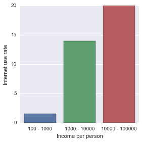
seaborn.factorplot(x="incomeperperson", y="internetuserate", data=sub2, kind="bar", ci=None)
plt.xlabel('Income per person')
plt.ylabel('Internet use rate')
Contingency table of observed counts
========================================
incomeperperson  100 - 1000  1000 - 10000  10000 - 100000
internetuserate
Less than 20             48            26               0
Greater than 20           4            60              45

Column percentages
========================================
incomeperperson  100 - 1000  1000 - 10000  10000 - 100000
internetuserate
Less than 20       0.923077      0.302326             0.0
Greater than 20    0.076923      0.697674             1.0

chi-square value, p value, expected counts
========================================
(92.356982887599486, 8.8091901262367566e-21, 2, array([[ 21.0273224 ,  34.77595628,  18.19672131],
       [ 30.9726776 ,  51.22404372,  26.80327869]]))

def recode(sub, recoding):
    sub['incomeperpersonV2'] = sub['incomeperperson'].map(recoding)

    # Header
    header = 'Comparing {0} and {1}'.format(*recoding.keys())
    print(header)
    print('=' * len(header) + '\n')

    # contingency table of observed counts
    ct = pandas.crosstab(sub['internetuserate'], sub['incomeperpersonV2'])
    print('Contingency table of observed counts')
    print('-' * len('Contingency table of observed counts'))
    print(str(ct) + '\n')

    # column percentages
    colsum = ct.sum(axis=0)
    colpct = ct/colsum
    print('Column percentages')
    print('-' * len('Column percentages'))
    print(str(colpct) + '\n')

    print('chi-square value, p value, expected counts')
    print('-' * len('chi-square value, p value, expected counts'))
    cs = scipy.stats.chi2_contingency(ct)
    print(str(cs) + '\n')

recode(sub1.copy(), {'100 - 1000': '100 - 1000', '1000 - 10000': '1000 - 10000'})
recode(sub1.copy(), {'100 - 1000': '100 - 1000', '10000 - 100000': '10000 - 100000'})
recode(sub1.copy(), {'1000 - 10000': '1000 - 10000', '10000 - 100000': '10000 - 100000'})
Comparing 100 - 1000 and 1000 - 10000
=====================================

Contingency table of observed counts
------------------------------------
incomeperpersonV2  100 - 1000  1000 - 10000
internetuserate
Less than 20               48            26
Greater than 20             4            60

Column percentages
------------------
incomeperpersonV2  100 - 1000  1000 - 10000
internetuserate
Less than 20         0.923077      0.302326
Greater than 20      0.076923      0.697674

chi-square value, p value, expected counts
------------------------------------------
(47.746562413123101, 4.8503395840347456e-12, 1, array([[ 27.88405797,  46.11594203],
       [ 24.11594203,  39.88405797]]))

Comparing 100 - 1000 and 10000 - 100000
=======================================

Contingency table of observed counts
------------------------------------
incomeperpersonV2  100 - 1000  10000 - 100000
internetuserate
Less than 20               48               0
Greater than 20             4              45

Column percentages
------------------
incomeperpersonV2  100 - 1000  10000 - 100000
internetuserate
Less than 20         0.923077             0.0
Greater than 20      0.076923             1.0

chi-square value, p value, expected counts
------------------------------------------
(78.577956612666426, 7.6902772386092302e-19, 1, array([[ 25.73195876,  22.26804124],
       [ 26.26804124,  22.73195876]]))

Comparing 1000 - 10000 and 10000 - 100000
=========================================

Contingency table of observed counts
------------------------------------
incomeperpersonV2  1000 - 10000  10000 - 100000
internetuserate
Less than 20                 26               0
Greater than 20              60              45

Column percentages
------------------
incomeperpersonV2  1000 - 10000  10000 - 100000
internetuserate
Less than 20           0.302326             0.0
Greater than 20        0.697674             1.0

chi-square value, p value, expected counts
------------------------------------------
(15.126175119023959, 0.00010055931031856319, 1, array([[ 17.06870229,   8.93129771],
       [ 68.93129771,  36.06870229]]))
Summary
With a Bonferroni adjustment of 0.05/3 = 0.017, there is a significant difference of internet use rate in all of my categories.
09 Aug 2016
Program and outputs
import pandas
import numpy
import statsmodels.formula.api as smf
import statsmodels.stats.multicomp as multi

data = pandas.read_csv('gapminder.csv')
print('Total number of countries: {0}'.format(len(data)))
Total number of countries: 213
# Convert numeric types
data['incomeperperson'] = pandas.to_numeric(data['incomeperperson'], errors='coerce')
data['internetuserate'] = pandas.to_numeric(data['internetuserate'], errors='coerce')

sub1 = data[['incomeperperson', 'internetuserate']].dropna()

print('Remaining number of countries: {0}'.format(len(sub1)))

# Since GDP per person isn't categorical data, I'm going to group it by magnitude first
groups = [pow(10, i) for i in range(2, 7)]
labels = ['{0} - {1}'.format(groups[index], i) for index, i in enumerate(groups[1:])]
sub1['incomeperperson'] = pandas.cut(sub1['incomeperperson'], groups, right=False, labels=labels)
Remaining number of countries: 183
model = smf.ols(formula='internetuserate ~ C(incomeperperson)', data=sub1).fit()
print(model.summary())
print('\n'*2)

print('Means for internet use rate by income per person')
m = sub1.groupby('incomeperperson').mean()
print(m)
print('\n'*2)

print('standard deviations for internet use rate by income per person')
sd = sub1.groupby('incomeperperson').std()
print(sd)
                            OLS Regression Results
==============================================================================
Dep. Variable:        internetuserate   R-squared:                       0.677
Model:                            OLS   Adj. R-squared:                  0.673
Method:                 Least Squares   F-statistic:                     188.3
Date:                Tue, 09 Aug 2016   Prob (F-statistic):           7.59e-45
Time:                        21:02:32   Log-Likelihood:                -765.55
No. Observations:                 183   AIC:                             1537.
Df Residuals:                     180   BIC:                             1547.
Df Model:                           2
Covariance Type:            nonrobust
==========================================================================================================
                                             coef    std err          t      P>|t|      [95.0% Conf. Int.]
----------------------------------------------------------------------------------------------------------
Intercept                                  8.3944      2.219      3.783      0.000         4.016    12.773
C(incomeperperson)[T.1000 - 10000]        24.2198      2.811      8.616      0.000        18.673    29.766
C(incomeperperson)[T.10000 - 100000]      62.8513      3.258     19.292      0.000        56.423    69.280
C(incomeperperson)[T.100000 - 1000000]          0          0        nan        nan             0         0
==============================================================================
Omnibus:                        3.852   Durbin-Watson:                   1.985
Prob(Omnibus):                  0.146   Jarque-Bera (JB):                3.473
Skew:                           0.326   Prob(JB):                        0.176
Kurtosis:                       3.175   Cond. No.                          inf
==============================================================================

Warnings:
[1] Standard Errors assume that the covariance matrix of the errors is correctly specified.
[2] The smallest eigenvalue is      0. This might indicate that there are
strong multicollinearity problems or that the design matrix is singular.


Means for internet use rate by income per person
                  internetuserate
incomeperperson
100 - 1000               8.394409
1000 - 10000            32.614232
10000 - 100000          71.245728
100000 - 1000000              NaN


standard deviations for internet use rate by income per person
                  internetuserate
incomeperperson
100 - 1000               8.328892
1000 - 10000            19.402752
10000 - 100000          15.484270
100000 - 1000000              NaN
 mc = multi.MultiComparison(sub1['internetuserate'], sub1['incomeperperson'])
 res = mc.tukeyhsd()
 print(res.summary())
     Multiple Comparison of Means - Tukey HSD,FWER=0.05
===========================================================
   group1        group2     meandiff  lower   upper  reject
-----------------------------------------------------------
 100 - 1000   1000 - 10000  24.2198  17.5765 30.8631  True
 100 - 1000  10000 - 100000 62.8513  55.1516  70.551  True
1000 - 10000 10000 - 100000 38.6315  31.6736 45.5894  True
-----------------------------------------------------------
Summary
A p-value of 7.59e-45 seems pretty significant, and in all comparisons, I was able to reject the null hypothesis. It seems certain that income per person has a very strong predictive effect on internet use rate.
30 Jun 2016
Program and outputs
%matplotlib inline
import pandas
import numpy
import seaborn
from matplotlib import pyplot

data = pandas.read_csv('gapminder.csv')
print('Total number of countries: {0}'.format(len(data)))
Total number of countries: 213
# Convert numeric types
data['incomeperperson'] = pandas.to_numeric(data['incomeperperson'], errors='coerce')

# Drop any countries with missing GPD
data = data[pandas.notnull(data['incomeperperson'])]

print('Remaining number of countries: {0}'.format(len(data['incomeperperson'])))
Remaining number of countries: 190
# Since GDP per person isn't categorical data, I'm going to group it by magnitude first
groups = [pow(10, i) for i in range(2, 7)]
labels = ['{0} - {1}'.format(groups[index], i) for index, i in enumerate(groups[1:])]
grouped = pandas.cut(data['incomeperperson'], groups, right=False, labels=labels)

grouped = grouped.astype('category')
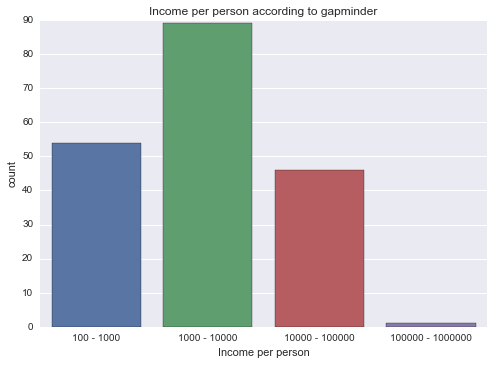
graph = seaborn.countplot(x=grouped)
pyplot.xlabel('Income per person')
pyplot.title('Income per person according to gapminder')

# Now do the above for all of my consumption types
types = [
    ('alcconsumption', 'Alcohol Consumption'),
    ('co2emissions', 'CO2 Emissions'),
    ('internetuserate', 'Internet Use Rate'),
    ('oilperperson', 'Oil per Person'),
    ('relectricperperson', 'Electricity per Person'),
]

# Convert to numeric
clean = data.copy()
for (key, name) in types:
    clean[key] = pandas.to_numeric(clean[key], errors='coerce')

def draw_distplot(series, name):
    # Drop NaNs
    series = series.dropna()

    # Draw a distplot
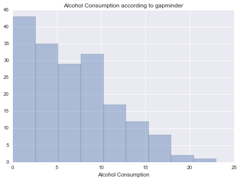
    graph = seaborn.distplot(series, kde=False)
    pyplot.xlabel(name)
    pyplot.title('{0} according to gapminder'.format(name))

def draw_regplot(data, y, name):
    # Draw a regplot
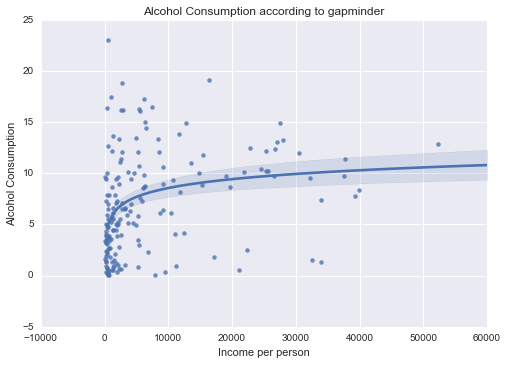
    seaborn.regplot(x='incomeperperson', y=y, data=data, logx=True)
    pyplot.xlabel('Income per person')
    pyplot.ylabel(name)
    pyplot.title('{0} according to gapminder'.format(name))

for (key, name) in types:
    draw_distplot(clean[key], name)
    draw_regplot(clean, key, name)
Alcohol consumption
Unimodal, skewed-right distribution.
CO2 Emissions
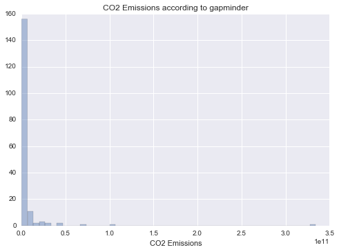
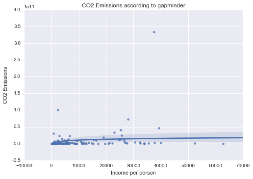
Unimodal, skewed-right distribution.
Internet Use Rate
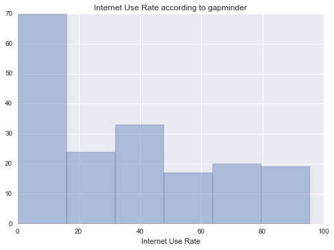
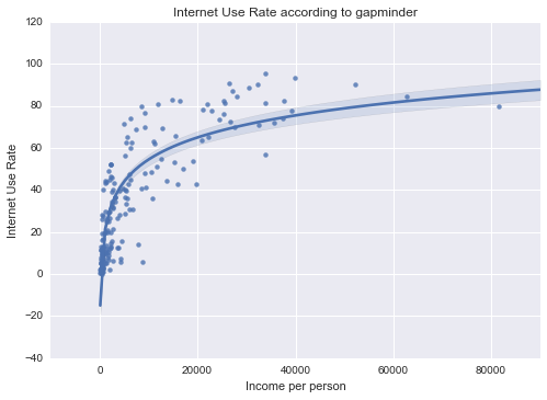
Unimodal, skewed-right distribution.
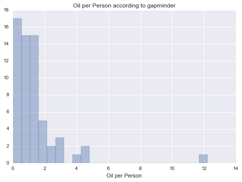
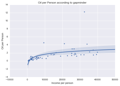
Oil per Person
Unimodal, skewed-right distribution.
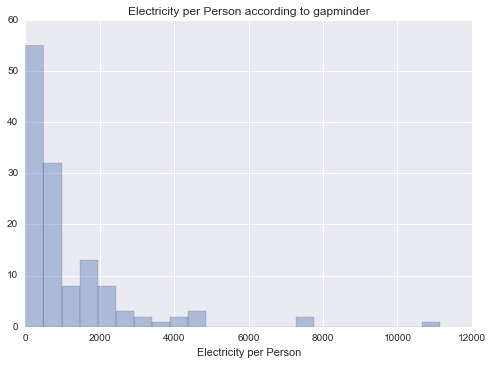
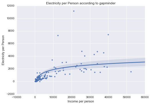
Electricity per Person
Unimodal, skewed-right distribution.
Summary
All of my measured variables were unimodal, and skewed-right. There was some correlation between my measured variables and Income per Person. In particular, Internet use rate was very closely correlated.
19 Jun 2016
Program and outputs
import pandas
import numpy

data = pandas.read_csv('gapminder.csv')
print('Total number of countries: {0}'.format(len(data)))
Total number of countries: 213
# Convert numeric types
data['incomeperperson'] = pandas.to_numeric(data['incomeperperson'], errors='coerce')

# Drop any countries with missing GPD
data = data[pandas.notnull(data['incomeperperson'])]

print('Remaining number of countries: {0}'.format(len(data['incomeperperson'])))
Remaining number of countries: 190
# Since GDP per person isn't categorical data, I'm going to group it by magnitude first
groups = [pow(10, i) for i in range(2, 7)]
labels = ['{0} - {1}'.format(groups[index], i) for index, i in enumerate(groups[1:])]
print('Groups: {0}'.format(labels))
Groups: ['100 - 1000', '1000 - 10000', '10000 - 100000', '100000 - 1000000']
grouped = pandas.cut(data['incomeperperson'], groups, right=False, labels=labels)
print('Counts for GDP per person, grouped by magnitude:')
print(grouped.value_counts(sort=False))
print('\nPercentages for GDP per person, grouped by magnitude:')
print(grouped.value_counts(sort=False, normalize=True))
Counts for GDP per person, grouped by magnitude:
100 - 1000          54
1000 - 10000        89
10000 - 100000      46
100000 - 1000000     1
Name: incomeperperson, dtype: int64

Percentages for GDP per person, grouped by magnitude:
100 - 1000          0.284211
1000 - 10000        0.468421
10000 - 100000      0.242105
100000 - 1000000    0.005263
Name: incomeperperson, dtype: float64
# Now do the above for all of my consumption types
types = [
    ('alcconsumption', 'Alcohol Consumption'),
    ('co2emissions', 'CO2 Emissions'),
    ('internetuserate', 'Internet Use Rate'),
    ('oilperperson', 'Oil per Person'),
    ('relectricperperson', 'Electricity per Person'),
]
def summarize(series, name):
    # Convert to numeric and drop NaNs
    series = pandas.to_numeric(series, errors='coerce')
    series.dropna(inplace=True)

    grouped = pandas.qcut(series, 4)

    print(name)
    print('-' * len(name))

    print('Counts for {0} grouped by percentile:'.format(name))
    print(grouped.value_counts(sort=False))

    print('Percentages for {0}, grouped by percentile (should probably be 25%)'.format(name))
    print(grouped.value_counts(sort=False, normalize=True))

for (key, name) in types:
    summarize(data[key], name)
    print('\n')
Alcohol Consumption
-------------------
Counts for Alcohol Consumption grouped by percentile:
[0.05, 2.73]       45
(2.73, 6.12]       45
(6.12, 10.035]     44
(10.035, 23.01]    45
Name: alcconsumption, dtype: int64
Percentages for Alcohol Consumption, grouped by percentile (should probably be 25%)
[0.05, 2.73]       0.251397
(2.73, 6.12]       0.251397
(6.12, 10.035]     0.245810
(10.035, 23.01]    0.251397
Name: alcconsumption, dtype: float64


CO2 Emissions
-------------
Counts for CO2 Emissions grouped by percentile:
[850666.667, 39924500]            45
(39924500, 234864666.667]         45
(234864666.667, 2138961000]       44
(2138961000, 334220872333.333]    45
Name: co2emissions, dtype: int64
Percentages for CO2 Emissions, grouped by percentile (should probably be 25%)
[850666.667, 39924500]            0.251397
(39924500, 234864666.667]         0.251397
(234864666.667, 2138961000]       0.245810
(2138961000, 334220872333.333]    0.251397
Name: co2emissions, dtype: float64


Internet Use Rate
-----------------
Counts for Internet Use Rate grouped by percentile:
[0.21, 9.949]         46
(9.949, 31.00438]     46
(31.00438, 55.646]    45
(55.646, 95.638]      46
Name: internetuserate, dtype: int64
Percentages for Internet Use Rate, grouped by percentile (should probably be 25%)
[0.21, 9.949]         0.251366
(9.949, 31.00438]     0.251366
(31.00438, 55.646]    0.245902
(55.646, 95.638]      0.251366
Name: internetuserate, dtype: float64


Oil per Person
--------------
Counts for Oil per Person grouped by percentile:
[0.0323, 0.505]    16
(0.505, 0.891]     15
(0.891, 1.593]     15
(1.593, 12.229]    15
Name: oilperperson, dtype: int64
Percentages for Oil per Person, grouped by percentile (should probably be 25%)
[0.0323, 0.505]    0.262295
(0.505, 0.891]     0.245902
(0.891, 1.593]     0.245902
(1.593, 12.229]    0.245902
Name: oilperperson, dtype: float64


Electricity per Person
----------------------
Counts for Electricity per Person grouped by percentile:
[0, 226.318]             33
(226.318, 609.335]       32
(609.335, 1484.703]      32
(1484.703, 11154.755]    33
Name: relectricperperson, dtype: int64
Percentages for Electricity per Person, grouped by percentile (should probably be 25%)
[0, 226.318]             0.253846
(226.318, 609.335]       0.246154
(609.335, 1484.703]      0.246154
(1484.703, 11154.755]    0.253846
Name: relectricperperson, dtype: float64
Summary
I began by dropping any rows where GDP per capita was missing, since I’m looking to eventually compare that to my various consumption categories. Then I showed the output of GDP grouped by magnitude (100 - 1000, 1000 - 10000, 10000 - 100000, 100000 - 1000000) since those gave me the most meaningful groupings.
Once that was done, I wanted to summarize each of my consumption types. For those I used the qcut method explained in this weeks lesson to break them each into quartiles.
Alcohol, CO2, and Internet use rate generally seem to have pretty thorough coverage of data (~180 countries), but oil and electricity per person are missing a lot more data. I’ll probably end up just using the first three types.
18 Jun 2016
Program and outputs
import pandas
import numpy

data = pandas.read_csv('gapminder.csv')
print('Total number of countries: {0}'.format(len(data)))
Total number of countries: 213
# Convert numeric types and drop NaNs
data['incomeperperson'] = pandas.to_numeric(data['incomeperperson'], errors='coerce')
data['incomeperperson'].dropna(inplace=True)

print('Remaining number of countries: {0}'.format(len(data['incomeperperson'])))
Remaining number of countries: 190
# Since GDP per person isn't categorical data, I'm going to group it by magnitude first
groups = [pow(10, i) for i in range(2, 7)]
labels = ['{0} - {1}'.format(groups[index], i) for index, i in enumerate(groups[1:])]
print('Groups: {0}'.format(labels))
Groups: ['100 - 1000', '1000 - 10000', '10000 - 100000', '100000 - 1000000']
grouped = pandas.cut(data['incomeperperson'], groups, right=False, labels=labels)
print('Counts for GDP per person, grouped by magnitude:')
print(grouped.value_counts(sort=False))
print('\nPercentages for GDP per person, grouped by magnitude:')
print(grouped.value_counts(sort=False, normalize=True))
Counts for GDP per person, grouped by magnitude:
100 - 1000          54
1000 - 10000        89
10000 - 100000      46
100000 - 1000000     1
Name: incomeperperson, dtype: int64

Percentages for GDP per person, grouped by magnitude:
100 - 1000          0.284211
1000 - 10000        0.468421
10000 - 100000      0.242105
100000 - 1000000    0.005263
Name: incomeperperson, dtype: float64
# Now do the above for all of my consumption types
types = [
    ('alcconsumption', 'Alcohol Consumption'),
    ('co2emissions', 'CO2 Emissions'),
    ('internetuserate', 'Internet Use Rate'),
    ('oilperperson', 'Oil per Person'),
    ('relectricperperson', 'Electricity per Person'),
]
def summarize(series, name):
    # Convert to numeric and drop NaNs
    series = pandas.to_numeric(series, errors='coerce')
    series.dropna(inplace=True)

    percentiles = numpy.linspace(0, 1, 5)
    groups = list(series.quantile(percentiles))
    labels = ['{0} - {1}'.format(groups[index], i) for index, i in enumerate(groups[1:])]
    grouped = pandas.cut(series, groups, right=False, labels=labels)

    print(name)
    print('-' * len(name))

    print('Counts for {0} grouped by percentile:'.format(name))
    print(grouped.value_counts(sort=False))

    print('Percentages for {0}, grouped by percentile (should probably be 25%)'.format(name))
    print(grouped.value_counts(sort=False, normalize=True))

for (key, name) in types:
    summarize(data[key], name)
    print('\n')
Alcohol Consumption
-------------------
Counts for Alcohol Consumption grouped by percentile:
0.03 - 2.625     47
2.625 - 5.92     45
5.92 - 9.925     48
9.925 - 23.01    46
Name: alcconsumption, dtype: int64
Percentages for Alcohol Consumption, grouped by percentile (should probably be 25%)
0.03 - 2.625     0.252688
2.625 - 5.92     0.241935
5.92 - 9.925     0.258065
9.925 - 23.01    0.247312
Name: alcconsumption, dtype: float64


CO2 Emissions
-------------
Counts for CO2 Emissions grouped by percentile:
132000.0 - 34846166.66666667             50
34846166.66666667 - 185901833.3333335    50
185901833.3333335 - 1846084166.666665    50
1846084166.666665 - 334220872333.333     49
Name: co2emissions, dtype: int64
Percentages for CO2 Emissions, grouped by percentile (should probably be 25%)
132000.0 - 34846166.66666667             0.251256
34846166.66666667 - 185901833.3333335    0.251256
185901833.3333335 - 1846084166.666665    0.251256
1846084166.666665 - 334220872333.333     0.246231
Name: co2emissions, dtype: float64


Internet Use Rate
-----------------
Counts for Internet Use Rate grouped by percentile:
0.210066325622776 - 9.999603951038267    48
9.999603951038267 - 31.81012075468915    48
31.81012075468915 - 56.41604586287351    48
56.41604586287351 - 95.6381132075472     47
Name: internetuserate, dtype: int64
Percentages for Internet Use Rate, grouped by percentile (should probably be 25%)
0.210066325622776 - 9.999603951038267    0.251309
9.999603951038267 - 31.81012075468915    0.251309
31.81012075468915 - 56.41604586287351    0.251309
56.41604586287351 - 95.6381132075472     0.246073
Name: internetuserate, dtype: float64


Oil per Person
--------------
Counts for Oil per Person grouped by percentile:
0.03228146619272 - 0.5325414918259135      16
0.5325414918259135 - 1.03246988375935      15
1.03246988375935 - 1.6227370046323601      16
1.6227370046323601 - 12.228644991426199    15
Name: oilperperson, dtype: int64
Percentages for Oil per Person, grouped by percentile (should probably be 25%)
0.03228146619272 - 0.5325414918259135      0.258065
0.5325414918259135 - 1.03246988375935      0.241935
1.03246988375935 - 1.6227370046323601      0.258065
1.6227370046323601 - 12.228644991426199    0.241935
Name: oilperperson, dtype: float64


Electricity per Person
----------------------
Counts for Electricity per Person grouped by percentile:
0.0 - 203.65210850945525                  34
203.65210850945525 - 597.1364359554304    34
597.1364359554304 - 1491.145248925905     34
1491.145248925905 - 11154.7550328078      33
Name: relectricperperson, dtype: int64
Percentages for Electricity per Person, grouped by percentile (should probably be 25%)
0.0 - 203.65210850945525                  0.251852
203.65210850945525 - 597.1364359554304    0.251852
597.1364359554304 - 1491.145248925905     0.251852
1491.145248925905 - 11154.7550328078      0.244444
Name: relectricperperson, dtype: float64
Conclusions
Since my data wasn’t categorical, it was a bit tricky to make it all work with value counts. However, that gave me the opportunity to learn a bit more about the pandas library, and how to create categories out of non-categorical data.
One thing I noticed pretty quickly, was that for both GDP and my various consumption variables, once the values started growing, they grow very quickly. For example, most of the alcohol consumption variables centered around 5 liters, but at the high end, it went as far as 23 liters.
