08 Nov 2016
Program and outputs
Data loading and cleaning
import numpy as np
import pandas as pandas
import seaborn
import statsmodels.api as sm
import statsmodels.formula.api as smf
from matplotlib import pyplot as plt

data = pandas.read_csv('gapminder.csv')
print('Total number of countries: {0}'.format(len(data)))
Total number of countries: 213
data['alcconsumption'] = pandas.to_numeric(data['alcconsumption'], errors='coerce')
data['femaleemployrate'] = pandas.to_numeric(data['femaleemployrate'], errors='coerce')
data['employrate'] = pandas.to_numeric(data['employrate'], errors='coerce')

sub1 = data[['alcconsumption', 'femaleemployrate', 'employrate']].dropna()
print('Total remaining countries: {0}'.format(len(sub1)))
Total remaining countries: 162
# Center quantitative IVs for regression analysis
sub1['femaleemployrate_c'] = sub1['femaleemployrate'] - sub1['femaleemployrate'].mean()
sub1['employrate_c'] = sub1['employrate'] - sub1['employrate'].mean()
sub1[['femaleemployrate_c', 'employrate_c']].mean()
femaleemployrate_c    2.434267e-15
employrate_c          3.640435e-15
dtype: float64
Single regression
# First order (linear) scatterplot
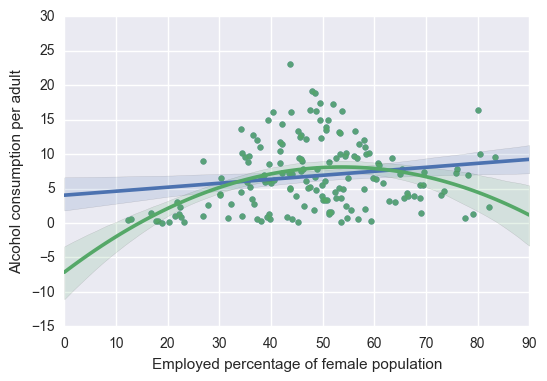
scat1 = seaborn.regplot(x='femaleemployrate', y='alcconsumption', scatter=True, data=sub1)

# Second order (polynomial) scatterplot
scat1 = seaborn.regplot(x='femaleemployrate', y='alcconsumption', scatter=True, order=2, data=sub1)
plt.xlabel('Employed percentage of female population')
plt.ylabel('Alcohol consumption per adult')
plt.show()

# Linear regression analysis
reg1 = smf.ols('alcconsumption ~ femaleemployrate_c', data=sub1).fit()
reg1.summary()
OLS Regression Results
| Dep. Variable: | alcconsumption | R-squared: | 0.029 |
| Model: | OLS | Adj. R-squared: | 0.023 |
| Method: | Least Squares | F-statistic: | 4.787 |
| Date: | Tue, 08 Nov 2016 | Prob (F-statistic): | 0.0301 |
| Time: | 11:20:44 | Log-Likelihood: | -487.57 |
| No. Observations: | 162 | AIC: | 979.1 |
| Df Residuals: | 160 | BIC: | 985.3 |
| Df Model: | 1 | | |
| Covariance Type: | nonrobust | | |
| coef | std err | t | P>|t| | [95.0% Conf. Int.] |
| Intercept | 6.8124 | 0.388 | 17.559 | 0.000 | 6.046 7.579 |
| femaleemployrate_c | 0.0578 | 0.026 | 2.188 | 0.030 | 0.006 0.110 |
| Omnibus: | 12.411 | Durbin-Watson: | 1.915 |
| Prob(Omnibus): | 0.002 | Jarque-Bera (JB): | 13.772 |
| Skew: | 0.713 | Prob(JB): | 0.00102 |
| Kurtosis: | 2.909 | Cond. No. | 14.7 |
# Quadratic (polynomial) regression analysis
reg2 = smf.ols('alcconsumption ~ femaleemployrate_c + I(femaleemployrate_c**2)', data=sub1).fit()
reg2.summary()
OLS Regression Results
| Dep. Variable: | alcconsumption | R-squared: | 0.135 |
| Model: | OLS | Adj. R-squared: | 0.125 |
| Method: | Least Squares | F-statistic: | 12.45 |
| Date: | Tue, 08 Nov 2016 | Prob (F-statistic): | 9.45e-06 |
| Time: | 11:20:45 | Log-Likelihood: | -478.17 |
| No. Observations: | 162 | AIC: | 962.3 |
| Df Residuals: | 159 | BIC: | 971.6 |
| Df Model: | 2 | | |
| Covariance Type: | nonrobust | | |
| coef | std err | t | P>|t| | [95.0% Conf. Int.] |
| Intercept | 7.9540 | 0.449 | 17.720 | 0.000 | 7.067 8.840 |
| femaleemployrate_c | 0.0605 | 0.025 | 2.419 | 0.017 | 0.011 0.110 |
| I(femaleemployrate_c ** 2) | -0.0053 | 0.001 | -4.423 | 0.000 | -0.008 -0.003 |
| Omnibus: | 9.022 | Durbin-Watson: | 1.930 |
| Prob(Omnibus): | 0.011 | Jarque-Bera (JB): | 9.369 |
| Skew: | 0.589 | Prob(JB): | 0.00924 |
| Kurtosis: | 3.024 | Cond. No. | 459. |
Multiple Regression
# Controlling for total employment rate
reg3 = smf.ols('alcconsumption ~ femaleemployrate_c + I(femaleemployrate_c**2) + employrate_c', data=sub1).fit()
reg3.summary()
OLS Regression Results
| Dep. Variable: | alcconsumption | R-squared: | 0.345 |
| Model: | OLS | Adj. R-squared: | 0.333 |
| Method: | Least Squares | F-statistic: | 27.79 |
| Date: | Tue, 08 Nov 2016 | Prob (F-statistic): | 1.73e-14 |
| Time: | 11:20:46 | Log-Likelihood: | -455.63 |
| No. Observations: | 162 | AIC: | 919.3 |
| Df Residuals: | 158 | BIC: | 931.6 |
| Df Model: | 3 | | |
| Covariance Type: | nonrobust | | |
| coef | std err | t | P>|t| | [95.0% Conf. Int.] |
| Intercept | 7.5561 | 0.396 | 19.092 | 0.000 | 6.774 8.338 |
| femaleemployrate_c | 0.3312 | 0.044 | 7.553 | 0.000 | 0.245 0.418 |
| I(femaleemployrate_c ** 2) | -0.0034 | 0.001 | -3.204 | 0.002 | -0.006 -0.001 |
| employrate_c | -0.4481 | 0.063 | -7.119 | 0.000 | -0.572 -0.324 |
| Omnibus: | 2.239 | Durbin-Watson: | 1.862 |
| Prob(Omnibus): | 0.326 | Jarque-Bera (JB): | 1.788 |
| Skew: | 0.205 | Prob(JB): | 0.409 |
| Kurtosis: | 3.311 | Cond. No. | 463. |
#Q-Q plot for normality
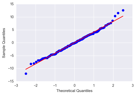
sm.qqplot(reg3.resid, line='r')
plt.show()

# simple plot of residuals
stdres = pandas.DataFrame(reg3.resid_pearson)
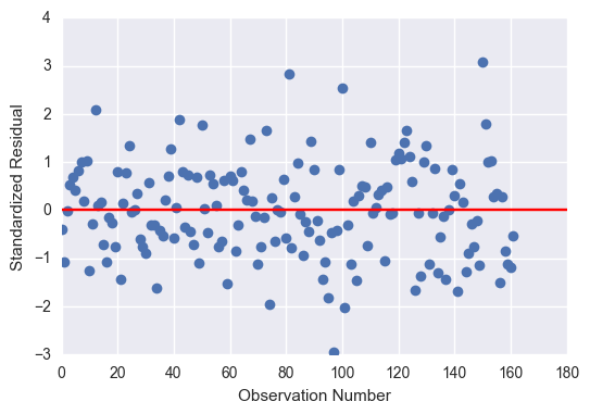
plt.plot(stdres, 'o', ls='None')
l = plt.axhline(y=0, color='r')
plt.ylabel('Standardized Residual')
plt.xlabel('Observation Number')
plt.show()

# additional regression diagnostic plots
fig2 = plt.figure(figsize=(12,8))
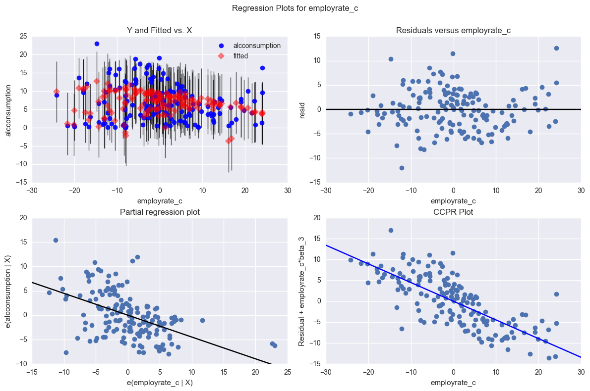
sm.graphics.plot_regress_exog(reg3,  "employrate_c", fig=fig2)
plt.show()

# leverage plot
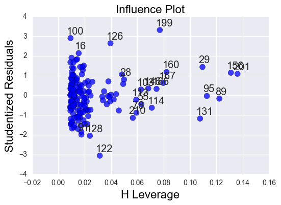
sm.graphics.influence_plot(reg3, size=8)
plt.show()


Summary
I started by analyzing the effect on female employment rate on alcohol consumption per adult. I found a significant (p = 0.0301) positive (coef = 0.0578) effect that explained a very small (r-squared = 0.029) portion of the data.
I then added a polynomial regression for female employment rate. I found a more significant (p = 9.45e-06) effect that explained a larger (r-squared = 0.135) portion of the data. Both of the variables individually are significant (p = 0.017 and p < 0.001) which confirms that the best fit line includes some curvature.
Assuming that the general employment rate would have an effect on the female employment rate, I decided to run my multiple regression, correcting for total employment rate. Again, my results were more significant (p = 1.73e-14) and had a greater effect (r-squared = 0.345). Again, all my variables were individually significant (p < 0.001, p = 0.002, p < 0.001).
Despite the overall significance of my explanatory variables, the total effect size was only 35%, so there are a fair number of residuals outside of 1 and 2 standard deviations. Nonetheless, the residuals with the greatest leverage were within 2 standard deviations, so I am confident saying that female employment rate, independent of the total employment rate, has a significant effect on alcohol consumption.
04 Nov 2016
Program and outputs
import numpy as np
import pandas as pandas
import seaborn
import statsmodels.api
import statsmodels.formula.api as smf
from matplotlib import pyplot as plt

data = pandas.read_csv('gapminder.csv')
print('Total number of countries: {0}'.format(len(data)))
Total number of countries: 213
data['incomeperperson'] = pandas.to_numeric(data['incomeperperson'], errors='coerce')
data['alcconsumption'] = pandas.to_numeric(data['alcconsumption'], errors='coerce')

clean = data[['incomeperperson', 'alcconsumption']].dropna()
print('Total remaining countries: {0}'.format(len(clean)))
Total remaining countries: 179
# Log based GDP is more meaningful
clean['log_income'] = np.log(clean['incomeperperson'])

centered = clean.copy()
centered['incomeperperson'] = centered['incomeperperson'] - centered['incomeperperson'].mean()
centered['log_income'] = centered['log_income'] - centered['log_income'].mean()

print('Mean GPD before centering:', clean['incomeperperson'].mean(), clean['log_income'].mean())
print('Mean GDP after centering:', centered['incomeperperson'].mean(), centered['log_income'].mean())
Mean GPD before centering: 7064.70280359 7.83342272135
Mean GDP after centering: 2.43886847403e-13 -7.93902498056e-16
# FORMULA: QUANT_RESPONSE ~ QUANT_EXPLANATORY
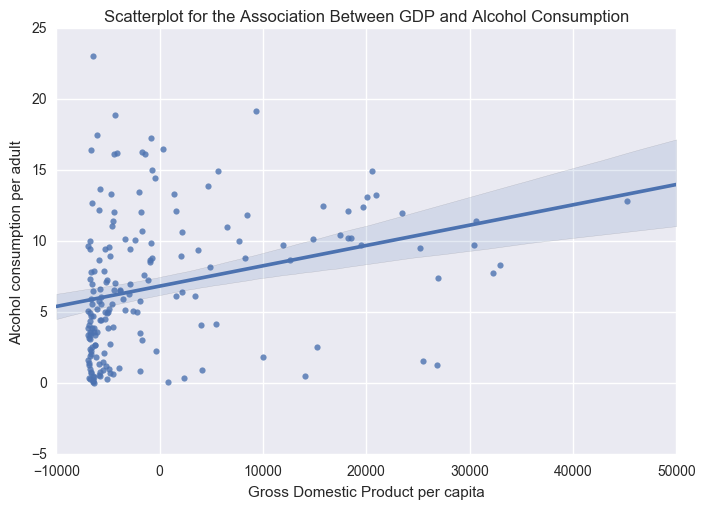
scat1 = seaborn.regplot(x="incomeperperson", y="alcconsumption", scatter=True, data=centered)
plt.xlabel('Gross Domestic Product per capita')
plt.ylabel('Alcohol consumption per adult')
plt.title('Scatterplot for the Association Between GDP and Alcohol Consumption')
print(scat1)

print ("OLS regression model for the association between urban rate and internet use rate")
reg1 = smf.ols('alcconsumption ~ incomeperperson', data=centered).fit()
print (reg1.summary())
OLS regression model for the association between urban rate and internet use rate
                            OLS Regression Results
==============================================================================
Dep. Variable:         alcconsumption   R-squared:                       0.087
Model:                            OLS   Adj. R-squared:                  0.082
Method:                 Least Squares   F-statistic:                     16.92
Date:                Fri, 04 Nov 2016   Prob (F-statistic):           5.96e-05
Time:                        11:33:42   Log-Likelihood:                -529.82
No. Observations:                 179   AIC:                             1064.
Df Residuals:                     177   BIC:                             1070.
Df Model:                           1
Covariance Type:            nonrobust
===================================================================================
                      coef    std err          t      P>|t|      [95.0% Conf. Int.]
-----------------------------------------------------------------------------------
Intercept           6.8409      0.351     19.493      0.000         6.148     7.534
incomeperperson     0.0001   3.48e-05      4.114      0.000      7.44e-05     0.000
==============================================================================
Omnibus:                       16.833   Durbin-Watson:                   2.036
Prob(Omnibus):                  0.000   Jarque-Bera (JB):               18.611
Skew:                           0.745   Prob(JB):                     9.09e-05
Kurtosis:                       3.524   Cond. No.                     1.01e+04
==============================================================================

# FORMULA: QUANT_RESPONSE ~ QUANT_EXPLANATORY
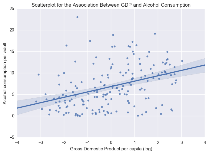
scat1 = seaborn.regplot(x="log_income", y="alcconsumption", scatter=True, data=centered)
plt.xlabel('Gross Domestic Product per capita (log)')
plt.ylabel('Alcohol consumption per adult')
plt.title('Scatterplot for the Association Between GDP and Alcohol Consumption')
print(scat1)

print ("OLS regression model for the association between urban rate and internet use rate")
reg1 = smf.ols('alcconsumption ~ log_income', data=centered).fit()
print (reg1.summary())
OLS regression model for the association between urban rate and internet use rate
                            OLS Regression Results
==============================================================================
Dep. Variable:         alcconsumption   R-squared:                       0.157
Model:                            OLS   Adj. R-squared:                  0.152
Method:                 Least Squares   F-statistic:                     32.90
Date:                Fri, 04 Nov 2016   Prob (F-statistic):           4.12e-08
Time:                        11:41:23   Log-Likelihood:                -522.73
No. Observations:                 179   AIC:                             1049.
Df Residuals:                     177   BIC:                             1056.
Df Model:                           1
Covariance Type:            nonrobust
==============================================================================
                 coef    std err          t      P>|t|      [95.0% Conf. Int.]
------------------------------------------------------------------------------
Intercept      6.8409      0.337     20.280      0.000         6.175     7.507
log_income     1.2525      0.218      5.736      0.000         0.822     1.683
==============================================================================
Omnibus:                       19.325   Durbin-Watson:                   1.998
Prob(Omnibus):                  0.000   Jarque-Bera (JB):               23.737
Skew:                           0.719   Prob(JB):                     7.01e-06
Kurtosis:                       4.056   Cond. No.                         1.54
==============================================================================

Summary
I performed a linear regression using GDP per capita as an explanatory variable for Alcohol consumption per adult. I also performed the same regression on log value for GDP per capita as I felt the results would be more meaningful.
GDP per capita
As an explanatory variable GDP doesn’t explain very much. The R-squared value is 0.087 or 8.7% of the variance in alcohol consumption. The p-value (5.96e-05) was below 0.05. The intercept and explanatory coeficients are 6.8409 and 0.0001, respectively.
Log value of GDP per capita
Log adjusted GDP is more correlated with alcohol consumption. The R-squared value is 0.157 or 15.7%. The p-value (4.12e-08) is lower as well. The intercept and explanatory coeficients are 6.8409 and 1.2525, respectively.
28 Oct 2016
Sample
The sample is from the GapMinder World dataset. It contains one year of data across 15 measures, including GDP per capita, life expectancy at birth and estimated HIV Prevalence for 215 areas (countries, geographical entities, semiautonomous territories and disputed territories). The GapMinder World dataset collects data from several sources, including the Institute for Health Metrics and Evaluation, US Census Bureau’s International Database, United Nations Statistics Division, and the World Bank.
Procedure
For GDP per capita, the dataset is based on GDP per capita, in fixed 2005 prices, and is adjusted for Purchasing Power Parities (PPPs), as calculated in the 2005 round of the International Comparison Program (ICP).
For life expectancy at birth, there were two main sources: a) Human Mortality Database and b) UN Population divisions World Population Prospects. As a first priority, data from Human Mortality Database (HMD) was used where available. For countries and/or time periods where the HMD did not have data, World Population Prospect was used, if available.
For estimated HIV Prevalence, data was gathered from a 2008 report from UNAIDS/WHO estimations on the current and previous state of the epidemic for most low and middle income countries.
Measures
2010 Gross Domestic Product per capita in constant 2000 US$. The
inflation but not the differences in the cost of living between countries has been taken into account.
2011 life expectancy at birth (years). The average number of years a newborn child would live if current mortality patterns were to stay the same.
2009 estimated HIV Prevalence % - (Ages 15-49). Estimated number of people living with HIV per 100 population of age group 15-49.
04 Sep 2016
Program and outputs
%matplotlib inline
import pandas
import numpy
import scipy
import seaborn
import statsmodels.formula.api as smf
from matplotlib import pyplot as plt

data = pandas.read_csv('gapminder.csv')
print('Total number of countries: {0}'.format(len(data)))
Total number of countries: 213
# Convert numeric types
data['incomeperperson'] = pandas.to_numeric(data['incomeperperson'], errors='coerce')
data['alcconsumption'] = pandas.to_numeric(data['alcconsumption'], errors='coerce')
data['lifeexpectancy'] = pandas.to_numeric(data['lifeexpectancy'], errors='coerce')

clean = data[['incomeperperson', 'alcconsumption', 'lifeexpectancy']].dropna()
print('Total remaining countries: {0}'.format(len(clean)))
Total remaining countries: 171
sub1 = clean[(clean['lifeexpectancy'] <= 70)]
sub2 = clean[(clean['lifeexpectancy'] > 70)]

def plot(data):
    seaborn.regplot(x="incomeperperson", y="alcconsumption", data=data)
    plt.xlabel('Income per Person')
    plt.ylabel('Alcohol Consumption')

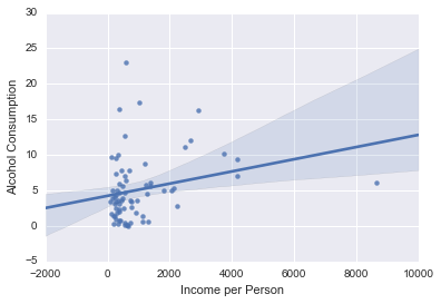
print('Association between income and alcohol consumption for those with a SHORTER life expectancy')
print(('correlation coefficient', 'p value'))
print(scipy.stats.pearsonr(sub1['incomeperperson'], sub1['alcconsumption']))
plot(sub1)

print('Association between income and alcohol consumption for those with a LONGER life expectancy')
print(('correlation coefficient', 'p value'))
print(scipy.stats.pearsonr(sub2['incomeperperson'], sub2['alcconsumption']))
plot(sub2)
Association between income and alcohol consumption for those with a SHORTER life expectancy
('correlation coefficient', 'p value')
(0.24564412558074125, 0.038937397029065977)

Association between income and alcohol consumption for those with a LONGER life expectancy
('correlation coefficient', 'p value')
(0.20396295528103475, 0.04180701551814929)

Summary
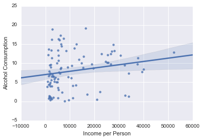
I ran a pearsonr correlation for income and alcohol consumption, moderated by countries with a SHORT (less than 70 years) life expectancy or a LONG (longer than 70 years) life expectancy. Despite having a significant P-value, the correlation coefficient is low enough that we can say that there is no correlation between income per person and alcohol consumption for either subgroup.
22 Aug 2016
Program and outputs
%matplotlib inline
import pandas
import numpy
import scipy
import seaborn
import matplotlib.pyplot as plt

data = pandas.read_csv('gapminder.csv')
print('Total number of countries: {0}'.format(len(data)))
Total number of countries: 213
# Convert numeric types
data['incomeperperson'] = pandas.to_numeric(data['incomeperperson'], errors='coerce')
data['alcconsumption'] = pandas.to_numeric(data['alcconsumption'], errors='coerce')
data['lifeexpectancy'] = pandas.to_numeric(data['lifeexpectancy'], errors='coerce')

clean = data[['incomeperperson', 'alcconsumption', 'lifeexpectancy']].dropna()
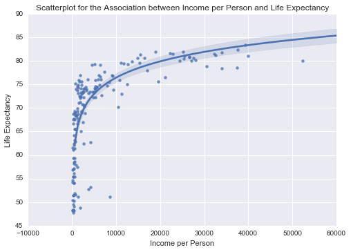
scat1 = seaborn.regplot(x='incomeperperson', y='lifeexpectancy', fit_reg=True, data=clean, logx=True)
plt.xlabel('Income per Person')
plt.ylabel('Life Expectancy')
plt.title('Scatterplot for the Association between Income per Person and Life Expectancy')

print('Association between Income per Person and Life Expectancy')
print(scipy.stats.pearsonr(clean['incomeperperson'], clean['lifeexpectancy']))

Association between Income per Person and Life Expectancy
(0.59534257610705288, 8.874239655396052e-18)
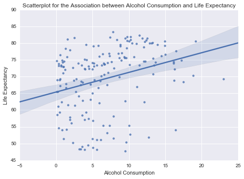
scat2 = seaborn.regplot(x='alcconsumption', y='lifeexpectancy', fit_reg=True, data=clean)
plt.xlabel('Alcohol Consumption')
plt.ylabel('Life Expectancy')
plt.title('Scatterplot for the Association between Alcohol Consumption and Life Expectancy')

print('Association between Alcohol Consumption and Life Expectancy')
print(scipy.stats.pearsonr(clean['alcconsumption'], clean['lifeexpectancy']))

Association between Alcohol Consumption and Life Expectancy
(0.29893173996914729, 7.1401036474160216e-05)
Summary
There is a significant difference between my two graphs, and the second one definitely doesn’t look significant.
There is a strong correlation between Income per Person and Life Expectancy. This has a very low p value, so we can say that this is significant.
There is a much weaker correlation between Alcohol Consumption and Life Expectancy, but the p value is still fairly low, so at least we can be confident about it.
