03 Feb 2017
Program and outputs
Data loading and cleaning
import pandas as pd

CSV_PATH = 'gapminder.csv'

data = pd.read_csv(CSV_PATH)
print('Total number of countries: {0}'.format(len(data)))
Total number of countries: 213
import numpy as np

PREDICTORS = [
    'incomeperperson', 'alcconsumption', 'armedforcesrate',
    'breastcancerper100th', 'co2emissions', 'femaleemployrate',
    'hivrate', 'internetuserate',
    'polityscore', 'relectricperperson', 'suicideper100th',
    'employrate', 'urbanrate'
]

clean = data.copy()

clean = clean.replace(r'\s+', np.NaN, regex=True)
clean = clean[PREDICTORS + ['lifeexpectancy']].dropna()

for key in PREDICTORS + ['lifeexpectancy']:
    clean[key] = pd.to_numeric(clean[key], errors='coerce')


clean = clean.dropna()

print('Countries remaining:', len(clean))
clean.head()
|
incomeperperson |
alcconsumption |
armedforcesrate |
breastcancerper100th |
co2emissions |
femaleemployrate |
hivrate |
internetuserate |
polityscore |
relectricperperson |
suicideper100th |
employrate |
urbanrate |
lifeexpectancy |
| 2 |
2231.993335 |
0.69 |
2.306817 |
23.5 |
2.932109e+09 |
31.700001 |
0.1 |
12.500073 |
2 |
590.509814 |
4.848770 |
50.500000 |
65.22 |
73.131 |
| 4 |
1381.004268 |
5.57 |
1.461329 |
23.1 |
2.483580e+08 |
69.400002 |
2.0 |
9.999954 |
-2 |
172.999227 |
14.554677 |
75.699997 |
56.70 |
51.093 |
| 6 |
10749.419238 |
9.35 |
0.560987 |
73.9 |
5.872119e+09 |
45.900002 |
0.5 |
36.000335 |
8 |
768.428300 |
7.765584 |
58.400002 |
92.00 |
75.901 |
| 7 |
1326.741757 |
13.66 |
2.618438 |
51.6 |
5.121967e+07 |
34.200001 |
0.1 |
44.001025 |
5 |
603.763058 |
3.741588 |
40.099998 |
63.86 |
74.241 |
| 9 |
25249.986061 |
10.21 |
0.486280 |
83.2 |
1.297009e+10 |
54.599998 |
0.1 |
75.895654 |
10 |
2825.391095 |
8.470030 |
61.500000 |
88.74 |
81.907 |
from sklearn import preprocessing
from sklearn.model_selection import train_test_split

predictors = clean[PREDICTORS].copy()
for key in PREDICTORS:
    predictors[key] = preprocessing.scale(predictors[key])

# split data into train and test sets
clus_train, clus_test = train_test_split(predictors, test_size=.3, random_state=123)
Running a k-means Cluster Analysis
from scipy.spatial.distance import cdist
from sklearn.cluster import KMeans

# k-means cluster analysis for 1-9 clusters
clusters = range(1,10)
meandist = []

for k in clusters:
    model = KMeans(n_clusters=k)
    model.fit(clus_train)
    clusassign=model.predict(clus_train)
    meandist.append(sum(np.min(cdist(clus_train, model.cluster_centers_, 'euclidean'), axis=1)) / clus_train.shape[0])
import matplotlib.pyplot as plt
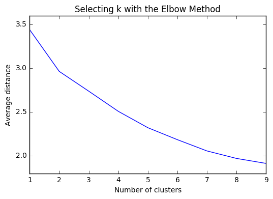
"""
Plot average distance from observations from the cluster centroid
to use the Elbow Method to identify number of clusters to choose
"""
plt.plot(clusters, meandist)
plt.xlabel('Number of clusters')
plt.ylabel('Average distance')
plt.title('Selecting k with the Elbow Method')
plt.show()
%matplotlib inline
from sklearn.decomposition import PCA
models = {}
# plot clusters
def plot(clus_train, model, n):
pca_2 = PCA(2)
plot_columns = pca_2.fit_transform(clus_train)
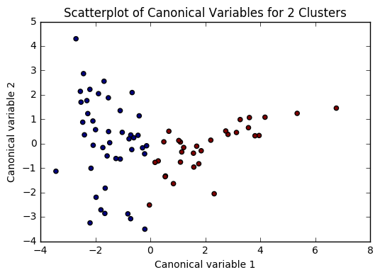
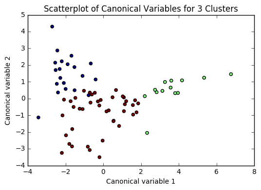
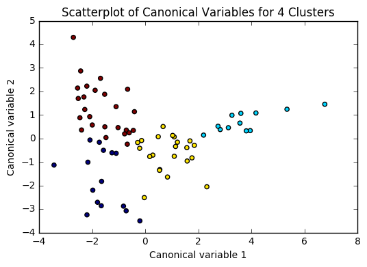
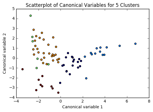
plt.scatter(x=plot_columns[:,0], y=plot_columns[:,1], c=model.labels_,)
plt.xlabel('Canonical variable 1')
plt.ylabel('Canonical variable 2')
plt.title('Scatterplot of Canonical Variables for {} Clusters'.format(n))
plt.show()
for n in range(2, 6):
# Interpret N cluster solution
models[n] = KMeans(n_clusters=n)
models[n].fit(clus_train)
clusassign = models[n].predict(clus_train)
plot(clus_train, models[n], n)
"""
BEGIN multiple steps to merge cluster assignment with clustering variables to examine
cluster variable means by cluster
"""
# create a unique identifier variable from the index for the
# cluster training data to merge with the cluster assignment variable
clus_train.reset_index(level=0, inplace=True)

# create a list that has the new index variable
cluslist = list(clus_train['index'])

# create a list of cluster assignments
labels = list(models[3].labels_)

# combine index variable list with cluster assignment list into a dictionary
newlist = dict(zip(cluslist, labels))

# convert newlist dictionary to a dataframe
newclus = pd.DataFrame.from_dict(newlist, orient='index')

# rename the cluster assignment column
newclus.columns = ['cluster']

# now do the same for the cluster assignment variable
# create a unique identifier variable from the index for the
# cluster assignment dataframe
# to merge with cluster training data
newclus.reset_index(level=0, inplace=True)

# merge the cluster assignment dataframe with the cluster training variable dataframe
# by the index variable
merged_train = pd.merge(clus_train, newclus, on='index')

# cluster frequencies
merged_train.cluster.value_counts()

"""
END multiple steps to merge cluster assignment with clustering variables to examine
cluster variable means by cluster
"""
Clustering variable means by cluster
clustergrp = merged_train.groupby('cluster').mean()
clustergrp
| cluster |
level_0 |
index |
incomeperperson |
alcconsumption |
armedforcesrate |
breastcancerper100th |
co2emissions |
femaleemployrate |
hivrate |
internetuserate |
polityscore |
relectricperperson |
suicideper100th |
employrate |
urbanrate |
| 0 |
31.450000 |
99.150000 |
-0.686916 |
-0.697225 |
0.013628 |
-0.755176 |
-0.240625 |
0.931895 |
0.372560 |
-0.957167 |
-0.641475 |
-0.647425 |
-0.317349 |
1.040447 |
-0.882169 |
| 1 |
41.615385 |
121.923077 |
1.995773 |
0.310344 |
-0.165620 |
1.510134 |
0.857540 |
0.479623 |
-0.354374 |
1.528231 |
0.568169 |
1.881545 |
0.000761 |
0.450520 |
0.964292 |
| 2 |
37.341463 |
108.902439 |
-0.300487 |
0.184597 |
0.150248 |
-0.104142 |
-0.126604 |
-0.668625 |
0.059176 |
-0.049347 |
0.147707 |
-0.221579 |
-0.096890 |
-0.704371 |
0.206884 |
# validate clusters in training data by examining cluster differences in life expectancy using ANOVA
# first have to merge life expectancy with clustering variables and cluster assignment data
le_data = clean['lifeexpectancy']

# split GPA data into train and test sets
le_train, le_test = train_test_split(le_data, test_size=.3, random_state=123)
le_train1 = pd.DataFrame(le_train)
le_train1.reset_index(level=0, inplace=True)
merged_train_all = pd.merge(le_train1, merged_train, on='index')
sub1 = merged_train_all[['lifeexpectancy', 'cluster']].dropna()
import statsmodels.formula.api as smf
import statsmodels.stats.multicomp as multi

lemod = smf.ols(formula='lifeexpectancy ~ C(cluster)', data=sub1).fit()
lemod.summary()
OLS Regression Results
| Dep. Variable: | lifeexpectancy | R-squared: | 0.471 |
| Model: | OLS | Adj. R-squared: | 0.457 |
| Method: | Least Squares | F-statistic: | 31.67 |
| Date: | Fri, 03 Feb 2017 | Prob (F-statistic): | 1.47e-10 |
| Time: | 16:40:56 | Log-Likelihood: | -243.38 |
| No. Observations: | 74 | AIC: | 492.8 |
| Df Residuals: | 71 | BIC: | 499.7 |
| Df Model: | 2 | | |
| Covariance Type: | nonrobust | | |
| coef | std err | t | P>|t| | [95.0% Conf. Int.] |
| Intercept | 62.3610 | 1.481 | 42.101 | 0.000 | 59.408 65.314 |
| C(cluster)[T.1] | 18.1989 | 2.360 | 7.712 | 0.000 | 13.493 22.905 |
| C(cluster)[T.2] | 10.2167 | 1.807 | 5.655 | 0.000 | 6.614 13.819 |
| Omnibus: | 11.030 | Durbin-Watson: | 1.942 |
| Prob(Omnibus): | 0.004 | Jarque-Bera (JB): | 11.189 |
| Skew: | -0.837 | Prob(JB): | 0.00372 |
| Kurtosis: | 3.908 | Cond. No. | 4.44 |
Means for Life Expectancy by cluster
sub1.groupby('cluster').mean()
| cluster |
lifeexpectancy |
| 0 |
62.361000 |
| 1 |
80.559923 |
| 2 |
72.577732 |
Standard deviations for Life Expectancy by cluster
sub1.groupby('cluster').std()
| cluster |
lifeexpectancy |
| 0 |
8.717742 |
| 1 |
1.450612 |
| 2 |
6.415368 |
mc1 = multi.MultiComparison(sub1['lifeexpectancy'], sub1['cluster'])
res1 = mc1.tukeyhsd()
res1.summary()
Multiple Comparison of Means - Tukey HSD,FWER=0.05
| group1 | group2 | meandiff | lower | upper | reject |
| 0 | 1 | 18.1989 | 12.5495 | 23.8483 | True |
| 0 | 2 | 10.2167 | 5.8917 | 14.5418 | True |
| 1 | 2 | -7.9822 | -13.0296 | -2.9348 | True |
Summary
Based on the plots of clusters based on Canonical variables, I proceeded with 3 clusters as my model. My three clusters were as follows:
- Cluster 0 - This looks like developing nations facing severe poverty. The urban rate is the lowest, combined with low income per person, and a high employment rate, looks like argicultural economies where everyone needs to work in order to remain at substinance income levels.
- Cluster 1 - This is very clearly a cluster of developed nations. There is a significantly higher incomeperperson, and higher consumption of things like CO2, residential electricity, and internet. There is also a much higher urban rate and polity score.
- Cluster 2 - This cluster is more similar to cluster 0, but with a trend towards urbanization. Income per person is higher, consumption is up, and the employment rate is way down.
There was a difference of about 10 years of mean life expectancy between each of my clusters, and the Tukey test considered each cluster as significant.
25 Jan 2017
Program and outputs
Data loading and cleaning
import pandas as pandas
from sklearn.model_selection import train_test_split
import numpy as np
import matplotlib.pylab as plt

CSV_PATH = 'gapminder.csv'

data = pandas.read_csv(CSV_PATH)
print('Total number of countries: {0}'.format(len(data)))
Total number of countries: 213
PREDICTORS = [
    'incomeperperson', 'alcconsumption', 'armedforcesrate',
    'breastcancerper100th', 'co2emissions', 'femaleemployrate',
    'hivrate', 'internetuserate',
    'polityscore', 'relectricperperson', 'suicideper100th',
    'employrate', 'urbanrate'
]

clean = data.copy()
for key in PREDICTORS + ['lifeexpectancy']:
    clean[key] = pandas.to_numeric(clean[key], errors='coerce')

clean = clean.dropna()

print('Countries remaining:', len(clean))
clean.head()
|
country |
incomeperperson |
alcconsumption |
armedforcesrate |
breastcancerper100th |
co2emissions |
femaleemployrate |
hivrate |
internetuserate |
lifeexpectancy |
oilperperson |
polityscore |
relectricperperson |
suicideper100th |
employrate |
urbanrate |
| 2 |
Algeria |
2231.993335 |
0.69 |
2.306817 |
23.5 |
2.932109e+09 |
31.700001 |
0.1 |
12.500073 |
73.131 |
.42009452521537 |
2.0 |
590.509814 |
4.848770 |
50.500000 |
65.22 |
| 4 |
Angola |
1381.004268 |
5.57 |
1.461329 |
23.1 |
2.483580e+08 |
69.400002 |
2.0 |
9.999954 |
51.093 |
|
-2.0 |
172.999227 |
14.554677 |
75.699997 |
56.70 |
| 6 |
Argentina |
10749.419238 |
9.35 |
0.560987 |
73.9 |
5.872119e+09 |
45.900002 |
0.5 |
36.000335 |
75.901 |
.635943800978195 |
8.0 |
768.428300 |
7.765584 |
58.400002 |
92.00 |
| 7 |
Armenia |
1326.741757 |
13.66 |
2.618438 |
51.6 |
5.121967e+07 |
34.200001 |
0.1 |
44.001025 |
74.241 |
|
5.0 |
603.763058 |
3.741588 |
40.099998 |
63.86 |
| 9 |
Australia |
25249.986061 |
10.21 |
0.486280 |
83.2 |
1.297009e+10 |
54.599998 |
0.1 |
75.895654 |
81.907 |
1.91302610912404 |
10.0 |
2825.391095 |
8.470030 |
61.500000 |
88.74 |
from sklearn import preprocessing

predictors = clean[PREDICTORS].copy()
for key in PREDICTORS:
    predictors[key] = preprocessing.scale(predictors[key])

targets = clean.lifeexpectancy

pred_train, pred_test, tar_train, tar_test = train_test_split(predictors, targets, test_size=.3, random_state=123)

print(pred_train.shape, pred_test.shape, tar_train.shape, tar_test.shape)
(74, 13) (33, 13) (74,) (33,)
from collections import OrderedDict
from sklearn.linear_model import LassoLarsCV

model = LassoLarsCV(cv=10, precompute=False).fit(pred_train, tar_train)

OrderedDict(sorted(zip(predictors.columns, model.coef_), key=lambda x:x[1], reverse=True))
OrderedDict([('internetuserate', 2.9741932507050883),
             ('incomeperperson', 1.5624998619776493),
             ('polityscore', 0.95348158080473089),
             ('urbanrate', 0.62824156642092388),
             ('alcconsumption', 0.0),
             ('armedforcesrate', 0.0),
             ('breastcancerper100th', 0.0),
             ('relectricperperson', 0.0),
             ('co2emissions', -0.065710252825883983),
             ('femaleemployrate', -0.16966106864470906),
             ('suicideper100th', -0.83797198915263182),
             ('employrate', -1.3086675757200679),
             ('hivrate', -3.6033945847485298)])
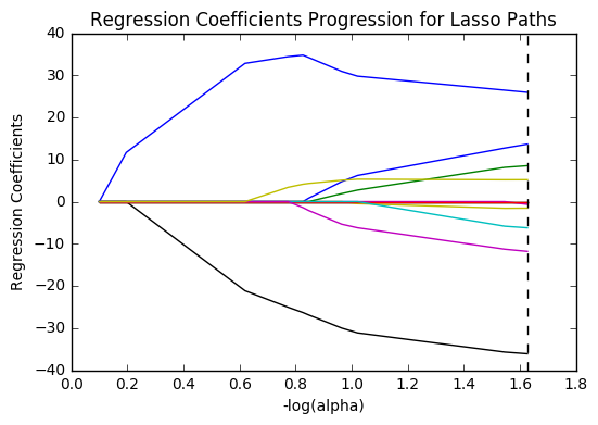
# plot coefficient progression
m_log_alphas = -np.log10(model.alphas_)
ax = plt.gca()
plt.plot(m_log_alphas, model.coef_path_.T)
plt.axvline(-np.log10(model.alpha_), linestyle='--', color='k', label='alpha CV')
plt.ylabel('Regression Coefficients')
plt.xlabel('-log(alpha)')
plt.title('Regression Coefficients Progression for Lasso Paths')
plt.show()
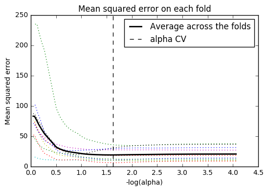
# plot mean square error for each fold
m_log_alphascv = -np.log10(model.cv_alphas_)
plt.figure()
plt.plot(m_log_alphascv, model.cv_mse_path_, ':')
plt.plot(m_log_alphascv, model.cv_mse_path_.mean(axis=-1), 'k', label='Average across the folds', linewidth=2)
plt.axvline(-np.log10(model.alpha_), linestyle='--', color='k', label='alpha CV')
plt.legend()
plt.xlabel('-log(alpha)')
plt.ylabel('Mean squared error')
plt.title('Mean squared error on each fold')
plt.show()
# MSE from training and test data
from sklearn.metrics import mean_squared_error
train_error = mean_squared_error(tar_train, model.predict(pred_train))
test_error = mean_squared_error(tar_test, model.predict(pred_test))
print('training data MSE')
print(train_error)
print('test data MSE')
print(test_error)
training data MSE
14.0227968412
test data MSE
22.9565114677
# R-square from training and test data
rsquared_train = model.score(pred_train, tar_train)
rsquared_test = model.score(pred_test, tar_test)
print('training data R-square')
print(rsquared_train)
print('test data R-square')
print(rsquared_test)
training data R-square
0.823964900718
test data R-square
0.658213145158
from collections import OrderedDict
from sklearn.linear_model import LassoLarsCV

model2 = LassoLarsCV(cv=10, precompute=False).fit(predictors, targets)

print('mse', mean_squared_error(targets, model2.predict(predictors)))
print('r-square', model2.score(predictors, targets))

OrderedDict(sorted(zip(predictors.columns, model2.coef_), key=lambda x:x[1], reverse=True))
mse 17.7754276093
r-square 0.766001466082

OrderedDict([('internetuserate', 2.6765897850358265),
             ('incomeperperson', 1.4881319407059432),
             ('urbanrate', 0.62065826306013672),
             ('polityscore', 0.49665728486271465),
             ('alcconsumption', 0.0),
             ('armedforcesrate', 0.0),
             ('breastcancerper100th', 0.0),
             ('co2emissions', 0.0),
             ('femaleemployrate', 0.0),
             ('relectricperperson', 0.0),
             ('suicideper100th', 0.0),
             ('employrate', -0.86922466889577155),
             ('hivrate', -3.6439368063365305)])
Summary
After running the Lasso regression, my model showed that HIV rate (-3.6) and internet use rate (3.0) were the most influential features in determining a country’s life expectancy. My model resulted in an R-square of 0.66 when run against the test dataset, down from 0.82 against the training set. This is a noticeable drop, but still high enough to suggest that these are reliable features.
Alcohol consumption, the armed forces rate, incidences of breast cancer, and residential electricity consumption ended up being reduced out of the model.
When I re-ran the model against the entire dataset (with ~100 records, the split dataset is incredibly small), it resulted in an R-square of 0.77, with the same features coming out on top. However, CO2 emissions, female employment rate, and sucide rates were all removed from the model.
Lasso regression seems like an incredibly useful tool to use at the start of data analysis, to identify features that are likely to produce useful results under other analysis methods.
19 Jan 2017
Program and outputs
Data loading and cleaning
import pandas as pandas
from sklearn.model_selection import train_test_split
from sklearn.ensemble import ExtraTreesClassifier, RandomForestClassifier
import sklearn.metrics
import numpy as np
import matplotlib.pylab as plt

CSV_PATH = 'gapminder.csv'

data = pandas.read_csv(CSV_PATH)
print('Total number of countries: {0}'.format(len(data)))
Total number of countries: 213
PREDICTORS = [
    'incomeperperson', 'alcconsumption', 'armedforcesrate',
    'breastcancerper100th', 'co2emissions', 'femaleemployrate',
    'hivrate', 'internetuserate', 'oilperperson',
    'polityscore', 'relectricperperson', 'suicideper100th',
    'employrate', 'urbanrate'
]

clean = data.copy()

clean = clean.replace(r'\s+', np.NaN, regex=True)
clean = clean[PREDICTORS + ['lifeexpectancy']].dropna()

for key in PREDICTORS + ['lifeexpectancy']:
    clean[key] = pandas.to_numeric(clean[key], errors='coerce', downcast='integer')

clean = clean.astype(int)
predictors = clean[PREDICTORS]
targets = clean.lifeexpectancy

pred_train, pred_test, tar_train, tar_test = train_test_split(predictors, targets, test_size=.4)

print(pred_train.shape, pred_test.shape, tar_train.shape, tar_test.shape)
(33, 14) (23, 14) (33,) (23,)
classifier=RandomForestClassifier(n_estimators=25)
classifier=classifier.fit(pred_train,tar_train)

predictions=classifier.predict(pred_test)

print('Confusion matrix:', sklearn.metrics.confusion_matrix(tar_test, predictions), sep='\n')
print('Accuracy score:', sklearn.metrics.accuracy_score(tar_test, predictions))
Confusion matrix:
[[0 0 0 0 0 0 0 1 0 0 0 0 0]
 [0 0 1 0 0 0 0 0 0 0 0 0 0]
 [0 0 0 0 1 0 0 0 0 0 0 0 0]
 [0 0 0 0 1 0 1 0 0 0 0 0 0]
 [0 0 1 0 3 0 2 0 0 0 0 0 0]
 [0 0 0 0 1 0 0 0 0 0 0 0 0]
 [0 0 0 0 0 0 0 0 0 0 0 0 0]
 [0 0 0 0 0 0 0 0 0 0 0 0 0]
 [0 0 0 0 0 0 0 0 0 0 0 2 0]
 [0 0 0 0 0 0 1 0 0 0 0 0 0]
 [0 0 0 0 0 0 0 0 0 1 0 4 0]
 [0 0 0 0 0 0 0 0 0 0 1 1 0]
 [0 0 0 0 0 0 0 0 0 0 0 1 0]]
Accuracy score: 0.173913043478
from table import table

# fit an Extra Trees model to the data
model = ExtraTreesClassifier()
model.fit(pred_train, tar_train)

# display the relative importance of each attribute
importances = list(zip(PREDICTORS, model.feature_importances_))
importances = sorted(importances, key=lambda x: x[1], reverse=True)

table(importances)
| urbanrate | 0.126317199412 |
| breastcancerper100th | 0.105117665487 |
| incomeperperson | 0.0948448657848 |
| internetuserate | 0.0771414112204 |
| employrate | 0.0757854973973 |
| suicideper100th | 0.073923975227 |
| alcconsumption | 0.0678999029417 |
| armedforcesrate | 0.0631145170619 |
| polityscore | 0.0601258137948 |
| co2emissions | 0.0597650190565 |
| femaleemployrate | 0.0555015579106 |
| oilperperson | 0.0544900713322 |
| relectricperperson | 0.0449603576248 |
| hivrate | 0.041012145749 |
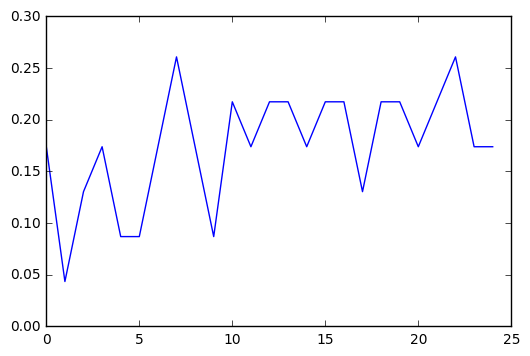
trees = range(25)
accuracy = np.zeros(25)

for idx in trees:
   classifier = RandomForestClassifier(n_estimators=idx + 1)
   classifier = classifier.fit(pred_train,tar_train)
   predictions = classifier.predict(pred_test)
   accuracy[idx] = sklearn.metrics.accuracy_score(tar_test, predictions)

plt.cla()
plt.plot(trees, accuracy)
Summary
The gapminder dataset continues to be fairly unimpressive with this form of analysis. The accuracy score of 0.17 indicates that the random forest has very little predictive power for determining life expectancy. I think there just aren’t enough remaining datapoints once the gapminder dataset has been cleaned up.
Urban rate, incidences of breast cancer, and income per person were the most important predictors, but having run the analysis a couple times I found that those numbers varied pretty wildly, nothing consistently stood out as a predictor.
Running the classifier with different numbers of trees was interesting. There was a general curve of improvement to accuracy, which seemed to level off around 10, but there’s enough variance even in that that I don’t think any meaningful conclusions can be drawn.
15 Jan 2017
Program and outputs
Data loading and cleaning
import pandas as pandas
from sklearn.model_selection import train_test_split
from sklearn.tree import DecisionTreeClassifier
import sklearn.metrics
import numpy as np

CSV_PATH = 'gapminder.csv'

data = pandas.read_csv(CSV_PATH)
print('Total number of countries: {0}'.format(len(data)))
Total number of countries: 213
PREDICTORS = [
    'incomeperperson', 'alcconsumption', 'armedforcesrate',
    'breastcancerper100th', 'co2emissions', 'femaleemployrate',
    'hivrate', 'internetuserate', 'oilperperson',
    'polityscore', 'relectricperperson', 'suicideper100th',
    'employrate', 'urbanrate'
]

clean = data.copy()

clean = clean.replace(r'\s+', np.NaN, regex=True)
clean = clean[PREDICTORS + ['lifeexpectancy']].dropna()

for key in PREDICTORS + ['lifeexpectancy']:
    clean[key] = pandas.to_numeric(clean[key], errors='coerce', downcast='integer')

clean = clean.astype(int)
predictors = clean[PREDICTORS]
targets = clean.lifeexpectancy

pred_train, pred_test, tar_train, tar_test = train_test_split(predictors, targets, test_size=.4)

print(pred_train.shape, pred_test.shape, tar_train.shape, tar_test.shape)
(33, 14) (23, 14) (33,) (23,)
Modeling and output
# Build model on training data
classifier = DecisionTreeClassifier()
classifier = classifier.fit(pred_train, tar_train)

predictions = classifier.predict(pred_test)

print('Confusion matrix:', sklearn.metrics.confusion_matrix(tar_test, predictions), sep='\n')
print('Accuracy score:', sklearn.metrics.accuracy_score(tar_test, predictions))
Confusion matrix:
[[0 0 0 0 0 0 0 0 0 0 0 0 0 0 0]
 [0 0 0 0 0 0 0 0 1 0 0 0 0 0 0]
 [0 0 0 0 0 0 1 0 0 1 0 0 0 0 0]
 [1 0 0 0 0 0 0 0 0 0 0 0 0 0 0]
 [0 0 0 0 0 0 1 0 0 1 0 0 0 0 0]
 [0 0 0 0 0 0 0 1 0 1 0 0 0 0 0]
 [1 0 0 0 0 0 1 2 0 0 0 0 0 0 0]
 [0 0 0 0 0 0 0 0 0 0 0 0 0 0 0]
 [0 0 0 0 0 0 0 0 0 0 0 0 0 0 0]
 [0 0 0 0 0 0 0 0 0 0 0 0 0 0 0]
 [0 0 0 0 0 0 0 0 0 0 0 0 0 0 0]
 [0 0 0 0 0 0 0 1 0 0 0 0 0 0 0]
 [0 0 0 0 0 0 0 0 0 0 2 1 1 0 0]
 [0 0 0 0 0 0 0 0 0 0 0 1 3 1 0]
 [0 0 0 0 0 0 0 0 0 0 0 0 1 0 0]]
Accuracy score: 0.130434782609
# Displaying the decision tree
from sklearn import tree
from io import StringIO
from IPython.display import Image
import pydotplus

out = StringIO()
tree.export_graphviz(classifier, out_file=out)
graph = pydotplus.graph_from_dot_data(out.getvalue())
Image(graph.create_png())
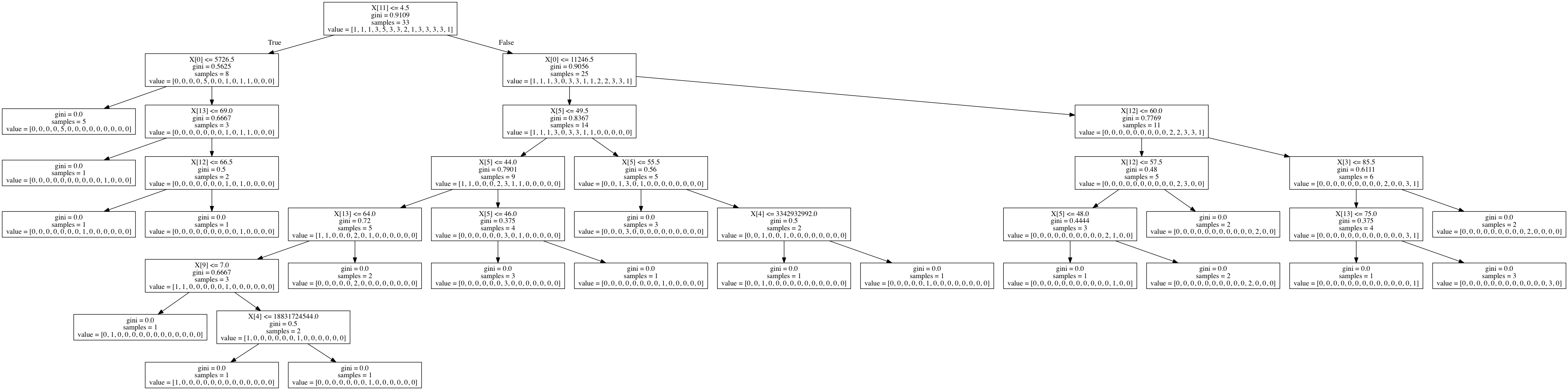
Summary
I was able to create a decision tree out of the gapminder dataset evaluating the conditions that contribute to life expectancy. A lot of data cleanup was required to generate this tree, as sklearn couldn&rsqu;t build a tree out of floats, which comprised most of my dataset.
I think the gapminder dataset is too small to build a meaningful decision tree. The accuracy score was 0.13 and the initial sample split was 8 and 25. The output is also incredibly hard to read. It would be nice to be able to replace X[0] with something like X[incomeperperson].
18 Nov 2016
Program and outputs
Data loading and cleaning
import numpy as np
import pandas as pandas
import seaborn
import statsmodels.api as sm
import statsmodels.formula.api as smf
from matplotlib import pyplot as plt

data = pandas.read_csv('gapminder.csv')
print('Total number of countries: {0}'.format(len(data)))
Total number of countries: 213
data['polityscore'] = pandas.to_numeric(data['polityscore'], errors='coerce')
data['internetuserate'] = pandas.to_numeric(data['internetuserate'], errors='coerce')
data['employrate'] = pandas.to_numeric(data['employrate'], errors='coerce')
data['urbanrate'] = pandas.to_numeric(data['urbanrate'], errors='coerce')
data['armedforcesrate'] = pandas.to_numeric(data['armedforcesrate'], errors='coerce')

# Since there are no categorical variables in the gapminder dataset,
# I'm creating one by grouping polity scores less than vs greater than 0.
labels = [0, 1]
data['polityscore_bins'] = pandas.cut(sub1['polityscore'], bins=2, labels=labels)
data['polityscore_bins'] = pandas.to_numeric(data['polityscore_bins'], errors='coerce')

sub1 = data[['polityscore', 'polityscore_bins', 'internetuserate', 'employrate', 'urbanrate', 'armedforcesrate']].dropna()

print('Total remaining countries: {0}'.format(len(sub1)))
Total remaining countries: 148
Logistic regression with no confounding variables
lreg1 = smf.logit(formula='polityscore_bins ~ internetuserate', data=sub1).fit()
lreg1.summary()
Logit Regression Results
| Dep. Variable: | polityscore_bins | No. Observations: | 148 |
| Model: | Logit | Df Residuals: | 146 |
| Method: | MLE | Df Model: | 1 |
| Date: | Fri, 18 Nov 2016 | Pseudo R-squ.: | 0.06948 |
| Time: | 17:03:41 | Log-Likelihood: | -86.076 |
| converged: | True | LL-Null: | -92.503 |
| | | LLR p-value: | 0.0003367 |
| coef | std err | z | P>|z| | [95.0% Conf. Int.] |
| Intercept | 0.0138 | 0.271 | 0.051 | 0.959 | -0.517 0.545 |
| internetuserate | 0.0255 | 0.008 | 3.298 | 0.001 | 0.010 0.041 |
def odds_ratios(lreg):
    params = lreg.params
    conf = lreg.conf_int()
    conf['OR'] = params
    conf.columns = ['Lower CI', 'Upper CI', 'OR']

    return np.exp(conf)

odds_ratios(lreg1)
|
Lower CI |
Upper CI |
OR |
| Intercept |
0.596194 |
1.724212 |
1.013886 |
| internetuserate |
1.010417 |
1.041558 |
1.025869 |
Logistic regression with confounding variables
lreg2 = smf.logit(formula='polityscore_bins ~ internetuserate + employrate + urbanrate + armedforcesrate', data=sub1).fit()
lreg2.summary()
Logit Regression Results
| Dep. Variable: | polityscore_bins | No. Observations: | 148 |
| Model: | Logit | Df Residuals: | 143 |
| Method: | MLE | Df Model: | 4 |
| Date: | Fri, 18 Nov 2016 | Pseudo R-squ.: | 0.1908 |
| Time: | 17:03:47 | Log-Likelihood: | -74.857 |
| converged: | True | LL-Null: | -92.503 |
| | | LLR p-value: | 4.046e-07 |
| coef | std err | z | P>|z| | [95.0% Conf. Int.] |
| Intercept | 4.2600 | 1.615 | 2.638 | 0.008 | 1.095 7.425 |
| internetuserate | 0.0364 | 0.012 | 3.015 | 0.003 | 0.013 0.060 |
| employrate | -0.0515 | 0.022 | -2.371 | 0.018 | -0.094 -0.009 |
| urbanrate | -0.0094 | 0.013 | -0.750 | 0.453 | -0.034 0.015 |
| armedforcesrate | -0.6771 | 0.185 | -3.651 | 0.000 | -1.041 -0.314 |
|
Lower CI |
Upper CI |
OR |
| Intercept |
2.990108 |
1677.028382 |
70.813105 |
| internetuserate |
1.012822 |
1.061937 |
1.037088 |
| employrate |
0.910171 |
0.991097 |
0.949772 |
| urbanrate |
0.966505 |
1.015320 |
0.990612 |
| armedforcesrate |
0.353227 |
0.730799 |
0.508072 |
Summary
My hypothesis was that internet use rate would be fairly well correlated with a nation’s polity score.
In my first logistic regression, I was surprised to find a high significance, but very low odds ratio (OR=1.03, 95% CI = 1.01-1.04, p=.001). Apparently, my hypothesis was incorrect.
After adjusting for potential confounding factors (employment rate, urbanrate, and armed forces rate), the odds of having a polity score greater than zero were almost half as likely for countries with a higher armed forces rate (OR=0.51, 95% CI = 0.35-0.73, p<0.001). None of the other factors were significantly associated with the polity score.