Assignment: Running a k-means Cluster Analysis
03 Feb 2017
Program and outputs
Data loading and cleaning
import pandas as pd

CSV_PATH = 'gapminder.csv'

data = pd.read_csv(CSV_PATH)
print('Total number of countries: {0}'.format(len(data)))
Total number of countries: 213
import numpy as np

PREDICTORS = [
    'incomeperperson', 'alcconsumption', 'armedforcesrate',
    'breastcancerper100th', 'co2emissions', 'femaleemployrate',
    'hivrate', 'internetuserate',
    'polityscore', 'relectricperperson', 'suicideper100th',
    'employrate', 'urbanrate'
]

clean = data.copy()

clean = clean.replace(r'\s+', np.NaN, regex=True)
clean = clean[PREDICTORS + ['lifeexpectancy']].dropna()

for key in PREDICTORS + ['lifeexpectancy']:
    clean[key] = pd.to_numeric(clean[key], errors='coerce')


clean = clean.dropna()

print('Countries remaining:', len(clean))
clean.head()
|
incomeperperson |
alcconsumption |
armedforcesrate |
breastcancerper100th |
co2emissions |
femaleemployrate |
hivrate |
internetuserate |
polityscore |
relectricperperson |
suicideper100th |
employrate |
urbanrate |
lifeexpectancy |
| 2 |
2231.993335 |
0.69 |
2.306817 |
23.5 |
2.932109e+09 |
31.700001 |
0.1 |
12.500073 |
2 |
590.509814 |
4.848770 |
50.500000 |
65.22 |
73.131 |
| 4 |
1381.004268 |
5.57 |
1.461329 |
23.1 |
2.483580e+08 |
69.400002 |
2.0 |
9.999954 |
-2 |
172.999227 |
14.554677 |
75.699997 |
56.70 |
51.093 |
| 6 |
10749.419238 |
9.35 |
0.560987 |
73.9 |
5.872119e+09 |
45.900002 |
0.5 |
36.000335 |
8 |
768.428300 |
7.765584 |
58.400002 |
92.00 |
75.901 |
| 7 |
1326.741757 |
13.66 |
2.618438 |
51.6 |
5.121967e+07 |
34.200001 |
0.1 |
44.001025 |
5 |
603.763058 |
3.741588 |
40.099998 |
63.86 |
74.241 |
| 9 |
25249.986061 |
10.21 |
0.486280 |
83.2 |
1.297009e+10 |
54.599998 |
0.1 |
75.895654 |
10 |
2825.391095 |
8.470030 |
61.500000 |
88.74 |
81.907 |
from sklearn import preprocessing
from sklearn.model_selection import train_test_split

predictors = clean[PREDICTORS].copy()
for key in PREDICTORS:
    predictors[key] = preprocessing.scale(predictors[key])

# split data into train and test sets
clus_train, clus_test = train_test_split(predictors, test_size=.3, random_state=123)
Running a k-means Cluster Analysis
from scipy.spatial.distance import cdist
from sklearn.cluster import KMeans

# k-means cluster analysis for 1-9 clusters
clusters = range(1,10)
meandist = []

for k in clusters:
    model = KMeans(n_clusters=k)
    model.fit(clus_train)
    clusassign=model.predict(clus_train)
    meandist.append(sum(np.min(cdist(clus_train, model.cluster_centers_, 'euclidean'), axis=1)) / clus_train.shape[0])
import matplotlib.pyplot as plt

"""
Plot average distance from observations from the cluster centroid
to use the Elbow Method to identify number of clusters to choose
"""
plt.plot(clusters, meandist)
plt.xlabel('Number of clusters')
plt.ylabel('Average distance')
plt.title('Selecting k with the Elbow Method')
plt.show()

%matplotlib inline

from sklearn.decomposition import PCA

models = {}

# plot clusters
def plot(clus_train, model, n):
    pca_2 = PCA(2)
    plot_columns = pca_2.fit_transform(clus_train)
    plt.scatter(x=plot_columns[:,0], y=plot_columns[:,1], c=model.labels_,)
    plt.xlabel('Canonical variable 1')
    plt.ylabel('Canonical variable 2')
    plt.title('Scatterplot of Canonical Variables for {} Clusters'.format(n))
    plt.show()

for n in range(2, 6):
    # Interpret N cluster solution
    models[n] = KMeans(n_clusters=n)
    models[n].fit(clus_train)
    clusassign = models[n].predict(clus_train)

    plot(clus_train, models[n], n)
"""
BEGIN multiple steps to merge cluster assignment with clustering variables to examine
cluster variable means by cluster
"""
# create a unique identifier variable from the index for the
# cluster training data to merge with the cluster assignment variable
clus_train.reset_index(level=0, inplace=True)

# create a list that has the new index variable
cluslist = list(clus_train['index'])

# create a list of cluster assignments
labels = list(models[3].labels_)

# combine index variable list with cluster assignment list into a dictionary
newlist = dict(zip(cluslist, labels))

# convert newlist dictionary to a dataframe
newclus = pd.DataFrame.from_dict(newlist, orient='index')

# rename the cluster assignment column
newclus.columns = ['cluster']

# now do the same for the cluster assignment variable
# create a unique identifier variable from the index for the
# cluster assignment dataframe
# to merge with cluster training data
newclus.reset_index(level=0, inplace=True)

# merge the cluster assignment dataframe with the cluster training variable dataframe
# by the index variable
merged_train = pd.merge(clus_train, newclus, on='index')

# cluster frequencies
merged_train.cluster.value_counts()

"""
END multiple steps to merge cluster assignment with clustering variables to examine
cluster variable means by cluster
"""
Clustering variable means by cluster
clustergrp = merged_train.groupby('cluster').mean()
clustergrp
| cluster |
level_0 |
index |
incomeperperson |
alcconsumption |
armedforcesrate |
breastcancerper100th |
co2emissions |
femaleemployrate |
hivrate |
internetuserate |
polityscore |
relectricperperson |
suicideper100th |
employrate |
urbanrate |
| 0 |
31.450000 |
99.150000 |
-0.686916 |
-0.697225 |
0.013628 |
-0.755176 |
-0.240625 |
0.931895 |
0.372560 |
-0.957167 |
-0.641475 |
-0.647425 |
-0.317349 |
1.040447 |
-0.882169 |
| 1 |
41.615385 |
121.923077 |
1.995773 |
0.310344 |
-0.165620 |
1.510134 |
0.857540 |
0.479623 |
-0.354374 |
1.528231 |
0.568169 |
1.881545 |
0.000761 |
0.450520 |
0.964292 |
| 2 |
37.341463 |
108.902439 |
-0.300487 |
0.184597 |
0.150248 |
-0.104142 |
-0.126604 |
-0.668625 |
0.059176 |
-0.049347 |
0.147707 |
-0.221579 |
-0.096890 |
-0.704371 |
0.206884 |
# validate clusters in training data by examining cluster differences in life expectancy using ANOVA
# first have to merge life expectancy with clustering variables and cluster assignment data
le_data = clean['lifeexpectancy']

# split GPA data into train and test sets
le_train, le_test = train_test_split(le_data, test_size=.3, random_state=123)
le_train1 = pd.DataFrame(le_train)
le_train1.reset_index(level=0, inplace=True)
merged_train_all = pd.merge(le_train1, merged_train, on='index')
sub1 = merged_train_all[['lifeexpectancy', 'cluster']].dropna()
import statsmodels.formula.api as smf
import statsmodels.stats.multicomp as multi

lemod = smf.ols(formula='lifeexpectancy ~ C(cluster)', data=sub1).fit()
lemod.summary()
OLS Regression Results
| Dep. Variable: | lifeexpectancy | R-squared: | 0.471 |
| Model: | OLS | Adj. R-squared: | 0.457 |
| Method: | Least Squares | F-statistic: | 31.67 |
| Date: | Fri, 03 Feb 2017 | Prob (F-statistic): | 1.47e-10 |
| Time: | 16:40:56 | Log-Likelihood: | -243.38 |
| No. Observations: | 74 | AIC: | 492.8 |
| Df Residuals: | 71 | BIC: | 499.7 |
| Df Model: | 2 | | |
| Covariance Type: | nonrobust | | |
| coef | std err | t | P>|t| | [95.0% Conf. Int.] |
| Intercept | 62.3610 | 1.481 | 42.101 | 0.000 | 59.408 65.314 |
| C(cluster)[T.1] | 18.1989 | 2.360 | 7.712 | 0.000 | 13.493 22.905 |
| C(cluster)[T.2] | 10.2167 | 1.807 | 5.655 | 0.000 | 6.614 13.819 |
| Omnibus: | 11.030 | Durbin-Watson: | 1.942 |
| Prob(Omnibus): | 0.004 | Jarque-Bera (JB): | 11.189 |
| Skew: | -0.837 | Prob(JB): | 0.00372 |
| Kurtosis: | 3.908 | Cond. No. | 4.44 |
Means for Life Expectancy by cluster
sub1.groupby('cluster').mean()
| cluster |
lifeexpectancy |
| 0 |
62.361000 |
| 1 |
80.559923 |
| 2 |
72.577732 |
Standard deviations for Life Expectancy by cluster
sub1.groupby('cluster').std()
| cluster |
lifeexpectancy |
| 0 |
8.717742 |
| 1 |
1.450612 |
| 2 |
6.415368 |
mc1 = multi.MultiComparison(sub1['lifeexpectancy'], sub1['cluster'])
res1 = mc1.tukeyhsd()
res1.summary()
Multiple Comparison of Means - Tukey HSD,FWER=0.05
| group1 | group2 | meandiff | lower | upper | reject |
| 0 | 1 | 18.1989 | 12.5495 | 23.8483 | True |
| 0 | 2 | 10.2167 | 5.8917 | 14.5418 | True |
| 1 | 2 | -7.9822 | -13.0296 | -2.9348 | True |
Summary
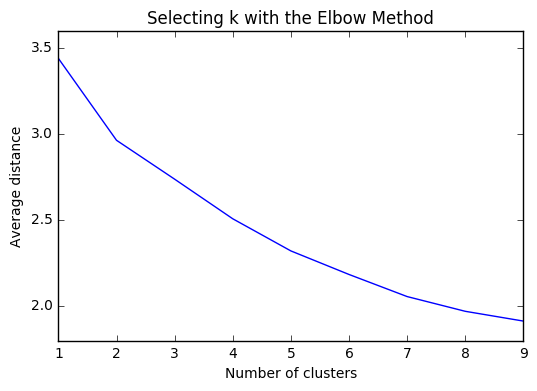
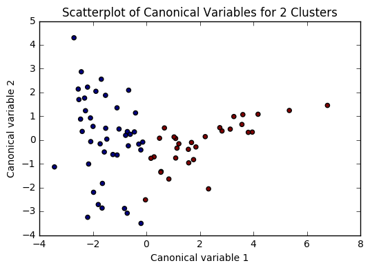
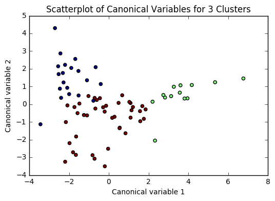
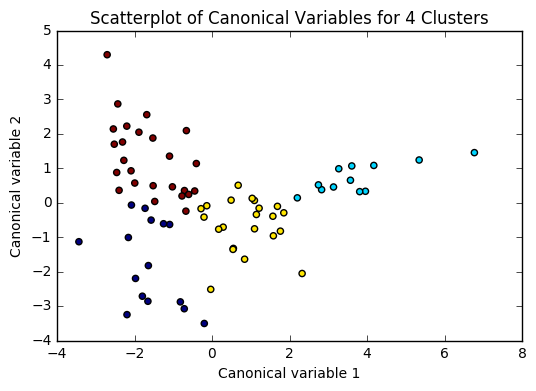
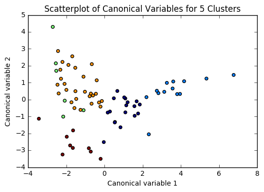
Based on the plots of clusters based on Canonical variables, I proceeded with 3 clusters as my model. My three clusters were as follows:
- Cluster 0 - This looks like developing nations facing severe poverty. The urban rate is the lowest, combined with low income per person, and a high employment rate, looks like argicultural economies where everyone needs to work in order to remain at substinance income levels.
- Cluster 1 - This is very clearly a cluster of developed nations. There is a significantly higher incomeperperson, and higher consumption of things like CO2, residential electricity, and internet. There is also a much higher urban rate and polity score.
- Cluster 2 - This cluster is more similar to cluster 0, but with a trend towards urbanization. Income per person is higher, consumption is up, and the employment rate is way down.
There was a difference of about 10 years of mean life expectancy between each of my clusters, and the Tukey test considered each cluster as significant.
