Assignment: Running a Lasso Regression Analysis
25 Jan 2017Program and outputs
Data loading and cleaning
import pandas as pandas
from sklearn.model_selection import train_test_split
import numpy as np
import matplotlib.pylab as plt

CSV_PATH = 'gapminder.csv'

data = pandas.read_csv(CSV_PATH)
print('Total number of countries: {0}'.format(len(data)))
Total number of countries: 213
PREDICTORS = [
    'incomeperperson', 'alcconsumption', 'armedforcesrate',
    'breastcancerper100th', 'co2emissions', 'femaleemployrate',
    'hivrate', 'internetuserate',
    'polityscore', 'relectricperperson', 'suicideper100th',
    'employrate', 'urbanrate'
]

clean = data.copy()
for key in PREDICTORS + ['lifeexpectancy']:
    clean[key] = pandas.to_numeric(clean[key], errors='coerce')

clean = clean.dropna()

print('Countries remaining:', len(clean))
clean.head()
Countries remaining: 107
| country | incomeperperson | alcconsumption | armedforcesrate | breastcancerper100th | co2emissions | femaleemployrate | hivrate | internetuserate | lifeexpectancy | oilperperson | polityscore | relectricperperson | suicideper100th | employrate | urbanrate | |
|---|---|---|---|---|---|---|---|---|---|---|---|---|---|---|---|---|
| 2 | Algeria | 2231.993335 | 0.69 | 2.306817 | 23.5 | 2.932109e+09 | 31.700001 | 0.1 | 12.500073 | 73.131 | .42009452521537 | 2.0 | 590.509814 | 4.848770 | 50.500000 | 65.22 |
| 4 | Angola | 1381.004268 | 5.57 | 1.461329 | 23.1 | 2.483580e+08 | 69.400002 | 2.0 | 9.999954 | 51.093 | -2.0 | 172.999227 | 14.554677 | 75.699997 | 56.70 | |
| 6 | Argentina | 10749.419238 | 9.35 | 0.560987 | 73.9 | 5.872119e+09 | 45.900002 | 0.5 | 36.000335 | 75.901 | .635943800978195 | 8.0 | 768.428300 | 7.765584 | 58.400002 | 92.00 |
| 7 | Armenia | 1326.741757 | 13.66 | 2.618438 | 51.6 | 5.121967e+07 | 34.200001 | 0.1 | 44.001025 | 74.241 | 5.0 | 603.763058 | 3.741588 | 40.099998 | 63.86 | |
| 9 | Australia | 25249.986061 | 10.21 | 0.486280 | 83.2 | 1.297009e+10 | 54.599998 | 0.1 | 75.895654 | 81.907 | 1.91302610912404 | 10.0 | 2825.391095 | 8.470030 | 61.500000 | 88.74 |
from sklearn import preprocessing

predictors = clean[PREDICTORS].copy()
for key in PREDICTORS:
    predictors[key] = preprocessing.scale(predictors[key])

targets = clean.lifeexpectancy

pred_train, pred_test, tar_train, tar_test = train_test_split(predictors, targets, test_size=.3, random_state=123)

print(pred_train.shape, pred_test.shape, tar_train.shape, tar_test.shape)
(74, 13) (33, 13) (74,) (33,)
from collections import OrderedDict
from sklearn.linear_model import LassoLarsCV

model = LassoLarsCV(cv=10, precompute=False).fit(pred_train, tar_train)

OrderedDict(sorted(zip(predictors.columns, model.coef_), key=lambda x:x[1], reverse=True))
OrderedDict([('internetuserate', 2.9741932507050883),
             ('incomeperperson', 1.5624998619776493),
             ('polityscore', 0.95348158080473089),
             ('urbanrate', 0.62824156642092388),
             ('alcconsumption', 0.0),
             ('armedforcesrate', 0.0),
             ('breastcancerper100th', 0.0),
             ('relectricperperson', 0.0),
             ('co2emissions', -0.065710252825883983),
             ('femaleemployrate', -0.16966106864470906),
             ('suicideper100th', -0.83797198915263182),
             ('employrate', -1.3086675757200679),
             ('hivrate', -3.6033945847485298)])
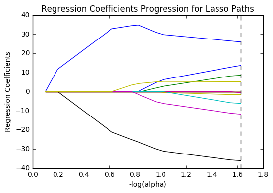
# plot coefficient progression
m_log_alphas = -np.log10(model.alphas_)
ax = plt.gca()
plt.plot(m_log_alphas, model.coef_path_.T)
plt.axvline(-np.log10(model.alpha_), linestyle='--', color='k', label='alpha CV')
plt.ylabel('Regression Coefficients')
plt.xlabel('-log(alpha)')
plt.title('Regression Coefficients Progression for Lasso Paths')
plt.show()

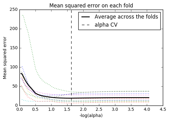
# plot mean square error for each fold
m_log_alphascv = -np.log10(model.cv_alphas_)
plt.figure()
plt.plot(m_log_alphascv, model.cv_mse_path_, ':')
plt.plot(m_log_alphascv, model.cv_mse_path_.mean(axis=-1), 'k', label='Average across the folds', linewidth=2)
plt.axvline(-np.log10(model.alpha_), linestyle='--', color='k', label='alpha CV')
plt.legend()
plt.xlabel('-log(alpha)')
plt.ylabel('Mean squared error')
plt.title('Mean squared error on each fold')
plt.show()

# MSE from training and test data
from sklearn.metrics import mean_squared_error
train_error = mean_squared_error(tar_train, model.predict(pred_train))
test_error = mean_squared_error(tar_test, model.predict(pred_test))
print('training data MSE')
print(train_error)
print('test data MSE')
print(test_error)
training data MSE
14.0227968412
test data MSE
22.9565114677
# R-square from training and test data
rsquared_train = model.score(pred_train, tar_train)
rsquared_test = model.score(pred_test, tar_test)
print('training data R-square')
print(rsquared_train)
print('test data R-square')
print(rsquared_test)
training data R-square
0.823964900718
test data R-square
0.658213145158
from collections import OrderedDict
from sklearn.linear_model import LassoLarsCV

model2 = LassoLarsCV(cv=10, precompute=False).fit(predictors, targets)

print('mse', mean_squared_error(targets, model2.predict(predictors)))
print('r-square', model2.score(predictors, targets))

OrderedDict(sorted(zip(predictors.columns, model2.coef_), key=lambda x:x[1], reverse=True))
mse 17.7754276093
r-square 0.766001466082

OrderedDict([('internetuserate', 2.6765897850358265),
             ('incomeperperson', 1.4881319407059432),
             ('urbanrate', 0.62065826306013672),
             ('polityscore', 0.49665728486271465),
             ('alcconsumption', 0.0),
             ('armedforcesrate', 0.0),
             ('breastcancerper100th', 0.0),
             ('co2emissions', 0.0),
             ('femaleemployrate', 0.0),
             ('relectricperperson', 0.0),
             ('suicideper100th', 0.0),
             ('employrate', -0.86922466889577155),
             ('hivrate', -3.6439368063365305)])
Summary
After running the Lasso regression, my model showed that HIV rate (-3.6) and internet use rate (3.0) were the most influential features in determining a country’s life expectancy. My model resulted in an R-square of 0.66 when run against the test dataset, down from 0.82 against the training set. This is a noticeable drop, but still high enough to suggest that these are reliable features.
Alcohol consumption, the armed forces rate, incidences of breast cancer, and residential electricity consumption ended up being reduced out of the model.
When I re-ran the model against the entire dataset (with ~100 records, the split dataset is incredibly small), it resulted in an R-square of 0.77, with the same features coming out on top. However, CO2 emissions, female employment rate, and sucide rates were all removed from the model.
Lasso regression seems like an incredibly useful tool to use at the start of data analysis, to identify features that are likely to produce useful results under other analysis methods.