Assignment: Test a Multiple Regression Model
08 Nov 2016Program and outputs
Data loading and cleaning
import numpy as np
import pandas as pandas
import seaborn
import statsmodels.api as sm
import statsmodels.formula.api as smf
from matplotlib import pyplot as plt

data = pandas.read_csv('gapminder.csv')
print('Total number of countries: {0}'.format(len(data)))
Total number of countries: 213
data['alcconsumption'] = pandas.to_numeric(data['alcconsumption'], errors='coerce')
data['femaleemployrate'] = pandas.to_numeric(data['femaleemployrate'], errors='coerce')
data['employrate'] = pandas.to_numeric(data['employrate'], errors='coerce')

sub1 = data[['alcconsumption', 'femaleemployrate', 'employrate']].dropna()
print('Total remaining countries: {0}'.format(len(sub1)))
Total remaining countries: 162
# Center quantitative IVs for regression analysis
sub1['femaleemployrate_c'] = sub1['femaleemployrate'] - sub1['femaleemployrate'].mean()
sub1['employrate_c'] = sub1['employrate'] - sub1['employrate'].mean()
sub1[['femaleemployrate_c', 'employrate_c']].mean()
femaleemployrate_c    2.434267e-15
employrate_c          3.640435e-15
dtype: float64
Single regression
# First order (linear) scatterplot
scat1 = seaborn.regplot(x='femaleemployrate', y='alcconsumption', scatter=True, data=sub1)

# Second order (polynomial) scatterplot
scat1 = seaborn.regplot(x='femaleemployrate', y='alcconsumption', scatter=True, order=2, data=sub1)
plt.xlabel('Employed percentage of female population')
plt.ylabel('Alcohol consumption per adult')
plt.show()
# Linear regression analysis
reg1 = smf.ols('alcconsumption ~ femaleemployrate_c', data=sub1).fit()
reg1.summary()
| Dep. Variable: | alcconsumption | R-squared: | 0.029 |
|---|---|---|---|
| Model: | OLS | Adj. R-squared: | 0.023 |
| Method: | Least Squares | F-statistic: | 4.787 |
| Date: | Tue, 08 Nov 2016 | Prob (F-statistic): | 0.0301 |
| Time: | 11:20:44 | Log-Likelihood: | -487.57 |
| No. Observations: | 162 | AIC: | 979.1 |
| Df Residuals: | 160 | BIC: | 985.3 |
| Df Model: | 1 | ||
| Covariance Type: | nonrobust |
| coef | std err | t | P>|t| | [95.0% Conf. Int.] | |
|---|---|---|---|---|---|
| Intercept | 6.8124 | 0.388 | 17.559 | 0.000 | 6.046 7.579 |
| femaleemployrate_c | 0.0578 | 0.026 | 2.188 | 0.030 | 0.006 0.110 |
| Omnibus: | 12.411 | Durbin-Watson: | 1.915 |
|---|---|---|---|
| Prob(Omnibus): | 0.002 | Jarque-Bera (JB): | 13.772 |
| Skew: | 0.713 | Prob(JB): | 0.00102 |
| Kurtosis: | 2.909 | Cond. No. | 14.7 |
# Quadratic (polynomial) regression analysis
reg2 = smf.ols('alcconsumption ~ femaleemployrate_c + I(femaleemployrate_c**2)', data=sub1).fit()
reg2.summary()
| Dep. Variable: | alcconsumption | R-squared: | 0.135 |
|---|---|---|---|
| Model: | OLS | Adj. R-squared: | 0.125 |
| Method: | Least Squares | F-statistic: | 12.45 |
| Date: | Tue, 08 Nov 2016 | Prob (F-statistic): | 9.45e-06 |
| Time: | 11:20:45 | Log-Likelihood: | -478.17 |
| No. Observations: | 162 | AIC: | 962.3 |
| Df Residuals: | 159 | BIC: | 971.6 |
| Df Model: | 2 | ||
| Covariance Type: | nonrobust |
| coef | std err | t | P>|t| | [95.0% Conf. Int.] | |
|---|---|---|---|---|---|
| Intercept | 7.9540 | 0.449 | 17.720 | 0.000 | 7.067 8.840 |
| femaleemployrate_c | 0.0605 | 0.025 | 2.419 | 0.017 | 0.011 0.110 |
| I(femaleemployrate_c ** 2) | -0.0053 | 0.001 | -4.423 | 0.000 | -0.008 -0.003 |
| Omnibus: | 9.022 | Durbin-Watson: | 1.930 |
|---|---|---|---|
| Prob(Omnibus): | 0.011 | Jarque-Bera (JB): | 9.369 |
| Skew: | 0.589 | Prob(JB): | 0.00924 |
| Kurtosis: | 3.024 | Cond. No. | 459. |
Multiple Regression
# Controlling for total employment rate
reg3 = smf.ols('alcconsumption ~ femaleemployrate_c + I(femaleemployrate_c**2) + employrate_c', data=sub1).fit()
reg3.summary()
| Dep. Variable: | alcconsumption | R-squared: | 0.345 |
|---|---|---|---|
| Model: | OLS | Adj. R-squared: | 0.333 |
| Method: | Least Squares | F-statistic: | 27.79 |
| Date: | Tue, 08 Nov 2016 | Prob (F-statistic): | 1.73e-14 |
| Time: | 11:20:46 | Log-Likelihood: | -455.63 |
| No. Observations: | 162 | AIC: | 919.3 |
| Df Residuals: | 158 | BIC: | 931.6 |
| Df Model: | 3 | ||
| Covariance Type: | nonrobust |
| coef | std err | t | P>|t| | [95.0% Conf. Int.] | |
|---|---|---|---|---|---|
| Intercept | 7.5561 | 0.396 | 19.092 | 0.000 | 6.774 8.338 |
| femaleemployrate_c | 0.3312 | 0.044 | 7.553 | 0.000 | 0.245 0.418 |
| I(femaleemployrate_c ** 2) | -0.0034 | 0.001 | -3.204 | 0.002 | -0.006 -0.001 |
| employrate_c | -0.4481 | 0.063 | -7.119 | 0.000 | -0.572 -0.324 |
| Omnibus: | 2.239 | Durbin-Watson: | 1.862 |
|---|---|---|---|
| Prob(Omnibus): | 0.326 | Jarque-Bera (JB): | 1.788 |
| Skew: | 0.205 | Prob(JB): | 0.409 |
| Kurtosis: | 3.311 | Cond. No. | 463. |
#Q-Q plot for normality
sm.qqplot(reg3.resid, line='r')
plt.show()

# simple plot of residuals
stdres = pandas.DataFrame(reg3.resid_pearson)
plt.plot(stdres, 'o', ls='None')
l = plt.axhline(y=0, color='r')
plt.ylabel('Standardized Residual')
plt.xlabel('Observation Number')
plt.show()

# additional regression diagnostic plots
fig2 = plt.figure(figsize=(12,8))
sm.graphics.plot_regress_exog(reg3,  "employrate_c", fig=fig2)
plt.show()

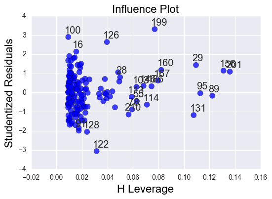
# leverage plot
sm.graphics.influence_plot(reg3, size=8)
plt.show()
Summary
I started by analyzing the effect on female employment rate on alcohol consumption per adult. I found a significant (p = 0.0301) positive (coef = 0.0578) effect that explained a very small (r-squared = 0.029) portion of the data.
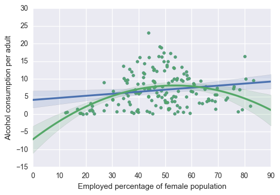
I then added a polynomial regression for female employment rate. I found a more significant (p = 9.45e-06) effect that explained a larger (r-squared = 0.135) portion of the data. Both of the variables individually are significant (p = 0.017 and p < 0.001) which confirms that the best fit line includes some curvature.
Assuming that the general employment rate would have an effect on the female employment rate, I decided to run my multiple regression, correcting for total employment rate. Again, my results were more significant (p = 1.73e-14) and had a greater effect (r-squared = 0.345). Again, all my variables were individually significant (p < 0.001, p = 0.002, p < 0.001).
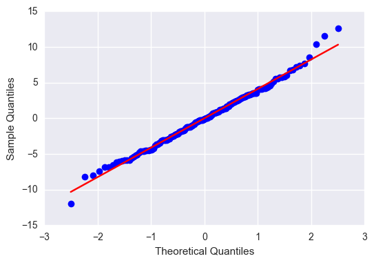
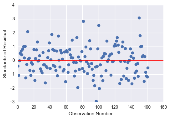
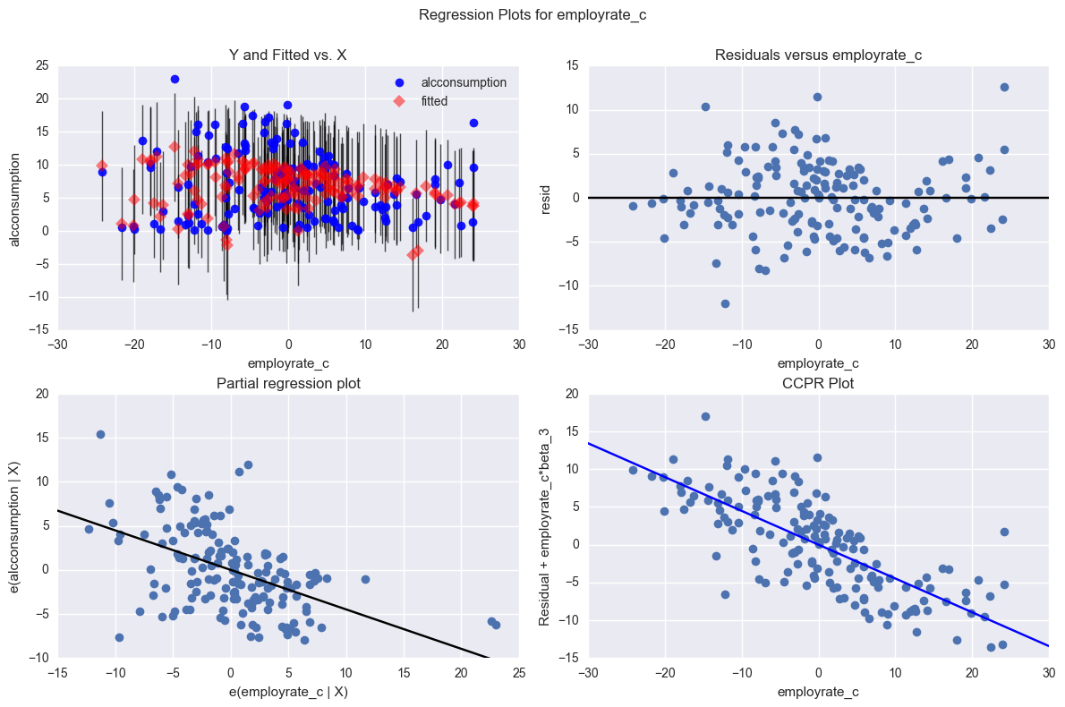
Despite the overall significance of my explanatory variables, the total effect size was only 35%, so there are a fair number of residuals outside of 1 and 2 standard deviations. Nonetheless, the residuals with the greatest leverage were within 2 standard deviations, so I am confident saying that female employment rate, independent of the total employment rate, has a significant effect on alcohol consumption.