Assignment: Test a Basic Linear Regression Model
04 Nov 2016Program and outputs
import numpy as np
import pandas as pandas
import seaborn
import statsmodels.api
import statsmodels.formula.api as smf
from matplotlib import pyplot as plt

data = pandas.read_csv('gapminder.csv')
print('Total number of countries: {0}'.format(len(data)))
Total number of countries: 213
data['incomeperperson'] = pandas.to_numeric(data['incomeperperson'], errors='coerce')
data['alcconsumption'] = pandas.to_numeric(data['alcconsumption'], errors='coerce')

clean = data[['incomeperperson', 'alcconsumption']].dropna()
print('Total remaining countries: {0}'.format(len(clean)))
Total remaining countries: 179
# Log based GDP is more meaningful
clean['log_income'] = np.log(clean['incomeperperson'])

centered = clean.copy()
centered['incomeperperson'] = centered['incomeperperson'] - centered['incomeperperson'].mean()
centered['log_income'] = centered['log_income'] - centered['log_income'].mean()

print('Mean GPD before centering:', clean['incomeperperson'].mean(), clean['log_income'].mean())
print('Mean GDP after centering:', centered['incomeperperson'].mean(), centered['log_income'].mean())
Mean GPD before centering: 7064.70280359 7.83342272135
Mean GDP after centering: 2.43886847403e-13 -7.93902498056e-16
# FORMULA: QUANT_RESPONSE ~ QUANT_EXPLANATORY
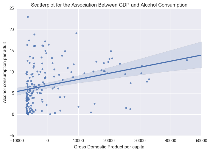
scat1 = seaborn.regplot(x="incomeperperson", y="alcconsumption", scatter=True, data=centered)
plt.xlabel('Gross Domestic Product per capita')
plt.ylabel('Alcohol consumption per adult')
plt.title('Scatterplot for the Association Between GDP and Alcohol Consumption')
print(scat1)

print ("OLS regression model for the association between urban rate and internet use rate")
reg1 = smf.ols('alcconsumption ~ incomeperperson', data=centered).fit()
print (reg1.summary())
OLS regression model for the association between urban rate and internet use rate
                            OLS Regression Results
==============================================================================
Dep. Variable:         alcconsumption   R-squared:                       0.087
Model:                            OLS   Adj. R-squared:                  0.082
Method:                 Least Squares   F-statistic:                     16.92
Date:                Fri, 04 Nov 2016   Prob (F-statistic):           5.96e-05
Time:                        11:33:42   Log-Likelihood:                -529.82
No. Observations:                 179   AIC:                             1064.
Df Residuals:                     177   BIC:                             1070.
Df Model:                           1
Covariance Type:            nonrobust
===================================================================================
                      coef    std err          t      P>|t|      [95.0% Conf. Int.]
-----------------------------------------------------------------------------------
Intercept           6.8409      0.351     19.493      0.000         6.148     7.534
incomeperperson     0.0001   3.48e-05      4.114      0.000      7.44e-05     0.000
==============================================================================
Omnibus:                       16.833   Durbin-Watson:                   2.036
Prob(Omnibus):                  0.000   Jarque-Bera (JB):               18.611
Skew:                           0.745   Prob(JB):                     9.09e-05
Kurtosis:                       3.524   Cond. No.                     1.01e+04
==============================================================================

# FORMULA: QUANT_RESPONSE ~ QUANT_EXPLANATORY
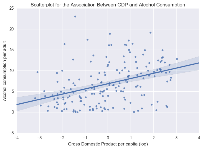
scat1 = seaborn.regplot(x="log_income", y="alcconsumption", scatter=True, data=centered)
plt.xlabel('Gross Domestic Product per capita (log)')
plt.ylabel('Alcohol consumption per adult')
plt.title('Scatterplot for the Association Between GDP and Alcohol Consumption')
print(scat1)

print ("OLS regression model for the association between urban rate and internet use rate")
reg1 = smf.ols('alcconsumption ~ log_income', data=centered).fit()
print (reg1.summary())
OLS regression model for the association between urban rate and internet use rate
                            OLS Regression Results
==============================================================================
Dep. Variable:         alcconsumption   R-squared:                       0.157
Model:                            OLS   Adj. R-squared:                  0.152
Method:                 Least Squares   F-statistic:                     32.90
Date:                Fri, 04 Nov 2016   Prob (F-statistic):           4.12e-08
Time:                        11:41:23   Log-Likelihood:                -522.73
No. Observations:                 179   AIC:                             1049.
Df Residuals:                     177   BIC:                             1056.
Df Model:                           1
Covariance Type:            nonrobust
==============================================================================
                 coef    std err          t      P>|t|      [95.0% Conf. Int.]
------------------------------------------------------------------------------
Intercept      6.8409      0.337     20.280      0.000         6.175     7.507
log_income     1.2525      0.218      5.736      0.000         0.822     1.683
==============================================================================
Omnibus:                       19.325   Durbin-Watson:                   1.998
Prob(Omnibus):                  0.000   Jarque-Bera (JB):               23.737
Skew:                           0.719   Prob(JB):                     7.01e-06
Kurtosis:                       4.056   Cond. No.                         1.54
==============================================================================

Summary
I performed a linear regression using GDP per capita as an explanatory variable for Alcohol consumption per adult. I also performed the same regression on log value for GDP per capita as I felt the results would be more meaningful.
GDP per capita
As an explanatory variable GDP doesn’t explain very much. The R-squared value is 0.087 or 8.7% of the variance in alcohol consumption. The p-value (5.96e-05) was below 0.05. The intercept and explanatory coeficients are 6.8409 and 0.0001, respectively.
Log value of GDP per capita
Log adjusted GDP is more correlated with alcohol consumption. The R-squared value is 0.157 or 15.7%. The p-value (4.12e-08) is lower as well. The intercept and explanatory coeficients are 6.8409 and 1.2525, respectively.